Chapter 4 Model Selection and Estimation
Chapter Preview. Chapters 2 and 3 have described how to fit parametric models to frequency and severity data, respectively. This chapter begins with the selection of models. To compare alternative parametric models, it is helpful to summarize data without reference to a specific parametric distribution. Section 4.1 describes nonparametric estimation, how we can use it for model comparisons and how it can be used to provide starting values for parametric procedures. The process of model selection is then summarized in Section 4.2. Although our focus is on data from continuous distributions, the same process can be used for discrete versions or data that come from a hybrid combination of discrete and continuous distributions.
Model selection and estimation are fundamental aspects of statistical modeling. To provide a flavor as to how they can be adapted to alternative sampling schemes, Section 4.3.1 describes estimation for grouped, censored and truncated data (following the Section 3.5 introduction). To see how they can be adapted to alternative models, the chapter closes with Section 4.4 on Bayesian inference, an alternative procedure where the (typically unknown) parameters are treated as random variables.
4.1 Nonparametric Inference
In this section, you learn how to:
- Estimate moments, quantiles, and distributions without reference to a parametric distribution
- Summarize the data graphically without reference to a parametric distribution
- Determine measures that summarize deviations of a parametric from a nonparametric fit
- Use nonparametric estimators to approximate parameters that can be used to start a parametric estimation procedure
4.1.1 Nonparametric Estimation
In Section 2.2 for frequency and Section 3.1 for severity, we learned how to summarize a distribution by computing means, variances, quantiles/percentiles, and so on. To approximate these summary measures using a dataset, one strategy is to:
- assume a parametric form for a distribution, such as a negative binomial for frequency or a gamma distribution for severity,
- estimate the parameters of that distribution, and then
- use the distribution with the estimated parameters to calculate the desired summary measure.
This is the parametricDistributional assumptions made on the population from which the data is drawn, with properties defined using parameters. approach. Another strategy is to estimate the desired summary measure directly from the observations without reference to a parametric model. Not surprisingly, this is known as the nonparametricNo distributional assumptions are made on the population from which the data is drawn. approach.
Let us start by considering the most basic type of sampling schemeHow the data is obtained from the population and what data is observed. and assume that observations are realizations from a set of random variables \(X_1, \ldots, X_n\) that are iidIndependent and identically distributed draws from an unknown population distribution \(F(\cdot)\). An equivalent way of saying this is that \(X_1, \ldots, X_n\), is a random sample (with replacement) from \(F(\cdot)\). To see how this works, we now describe nonparametric estimators of many important measures that summarize a distribution.
4.1.1.1 Moment Estimators
We learned how to define moments in Section 2.2.2 for frequency and Section 3.1.1 for severity. In particular, the \(k\)-th moment, \(\mathrm{E~}[X^k] = \mu^{\prime}_k\), summarizes many aspects of the distribution for different choices of \(k\). Here, \(\mu^{\prime}_k\) is sometimes called the \(k\)th population moment to distinguish it from the \(k\)th sample moment, \[ \frac{1}{n} \sum_{i=1}^n X_i^k , \] which is the corresponding nonparametric estimator. In typical applications, \(k\) is a positive integer, although it need not be in theory.
An important special case is the first moment where \(k=1\). In this case, the prime symbol (\(\prime\)) and the \(1\) subscript are usually dropped and one uses \(\mu=\mu^{\prime}_1\) to denote the population mean, or simply the mean. The corresponding sample estimator for \(\mu\) is called the sample mean, denoted with a bar on top of the random variable:
\[ \overline{X} =\frac{1}{n} \sum_{i=1}^n X_i . \]
Another type of summary measure of interest is the \(k\)-th central moment, \(\mathrm{E~} [(X-\mu)^k] = \mu_k\). (Sometimes, \(\mu^{\prime}_k\) is called the \(k\)-th raw moment to distinguish it from the central moment \(\mu_k\).). A nonparametric, or sample, estimator of \(\mu_k\) is \[ \frac{1}{n} \sum_{i=1}^n \left(X_i - \overline{X}\right)^k . \] The second central moment (\(k=2\)) is an important case for which we typically assign a new symbol, \(\sigma^2 = \mathrm{E~} [(X-\mu)^2]\), known as the variance. Properties of the sample moment estimator of the variance such as \(n^{-1}\sum_{i=1}^n \left(X_i - \overline{X}\right)^2\) have been studied extensively but is not the only possible estimator. The most widely used version is one where the effective sample size is reduced by one, and so we define \[ s^2 = \frac{1}{n-1} \sum_{i=1}^n \left(X_i - \overline{X}\right)^2. \]
Dividing by \(n-1\) instead of \(n\) matters little when you have a large sample size \(n\) as is common in insurance applications. The sample variance estimator \(s^2\) is unbiasedAn estimator that has no bias, that is, the expected value of an estimator equals the parameter being estimated. in the sense that \(\mathrm{E~} [s^2] = \sigma^2\), a desirable property particularly when interpreting results of an analysis.
4.1.1.2 Empirical Distribution Function
We have seen how to compute nonparametric estimators of the \(k\)th moment \(\mathrm{E~} [X^k]\). In the same way, for any known function \(\mathrm{g}(\cdot)\), we can estimate \(\mathrm{E~} [\mathrm{g}(X)]\) using \(n^{-1}\sum_{i=1}^n \mathrm{g}(X_i)\).
Now consider the function \(\mathrm{g}(X) = I(X \le x)\) for a fixed \(x\). Here, the notation \(I(\cdot)\) is the indicatorA categorical variable that has only two groups. the numerical values are usually taken to be one to indicate the presence of an attribute, and zero otherwise. another name for a binary variable. function; it returns 1 if the event \((\cdot)\) is true and 0 otherwise. Note that now the random variable \(\mathrm{g}(X)\) has Bernoulli distribution (a binomial distribution with \(n=1\)). We can use this distribution to readily calculate quantities such as the mean and the variance. For example, for this choice of \(\mathrm{g}(\cdot)\), the expected value is \(\mathrm{E~} [I(X \le x)] = \Pr(X \le x) = F(x)\), the distribution function evaluated at \(x\). Using the analog principle, we define the nonparametric estimator of the distribution function
\[
\begin{aligned}
F_n(x)
&= \frac{1}{n} \sum_{i=1}^n I\left(X_i \le x\right) \\
&= \frac{\text{number of observations less than or equal to }x}{n} .
\end{aligned}
\]
As \(F_n(\cdot)\) is based on only observations and does not assume a parametric family for the distribution, it is nonparametric and also known as the empirical distribution functionThe empirical distribution is a non-parametric estimate of the underlying distribution of a random variable. it directly uses the data observations to construct the distribution, with each observed data point in a size-n sample having probability 1/n. . It is also known as the empirical cumulative distribution function and, in R, one can use the ecdf(.) function to compute it.
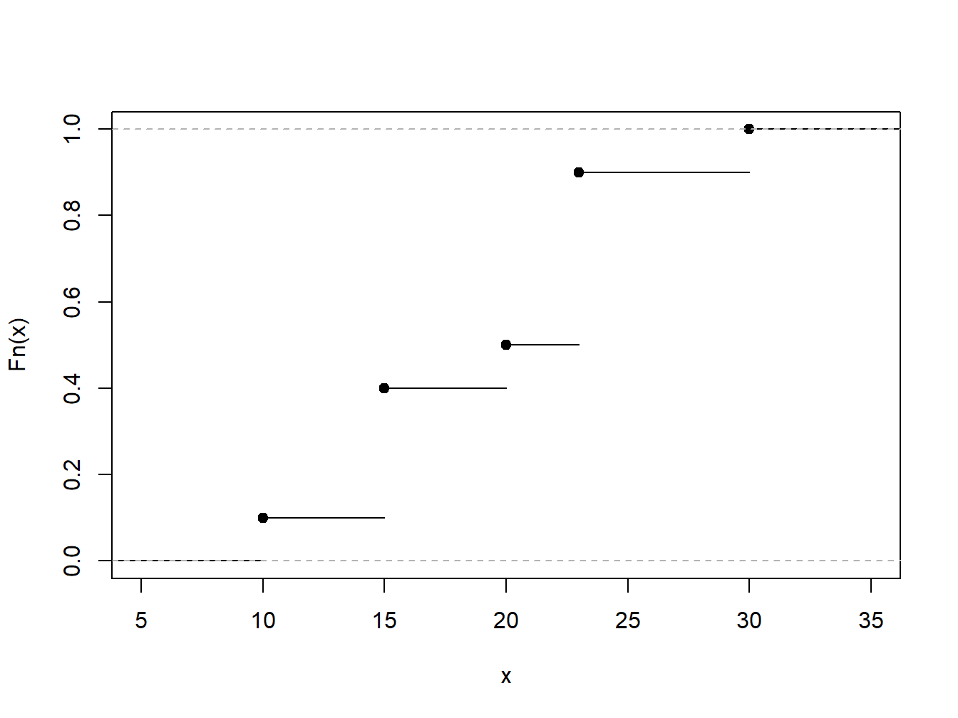
Example 4.1.1. Toy Data Set. To illustrate, consider a fictitious, or “toy,” data set of \(n=10\) observations. Determine the empirical distribution function.
\[ {\small \begin{array}{c|cccccccccc} \hline i &1&2&3&4&5&6&7&8&9&10 \\ X_i& 10 &15 &15 &15 &20 &23 &23 &23 &23 &30\\ \hline \end{array} } \]
Show Example Solution
4.1.1.3 Quartiles, Percentiles and Quantiles
We have already seen in Section 3.1.1 the median50th percentile of a definition, or middle value where half of the distribution lies below, which is the number such that approximately half of a data set is below (or above) it. The first quartileThe 25th percentile; the number such that approximately 25% of the data is below it. is the number such that approximately 25% of the data is below it and the third quartileThe 75th percentile; the number such that approximately 75% of the data is below it. is the number such that approximately 75% of the data is below it. A \(100p\) percentileA 100p-th percentile is the number such that 100 times p percent of the data is below it. is the number such that \(100 \times p\) percent of the data is below it.
To generalize this concept, consider a distribution function \(F(\cdot)\), which may or may not be continuous, and let \(q\) be a fraction so that \(0<q<1\). We want to define a quantileThe q-th quantile is the point(s) at which the distribution function is equal to q, i.e. the inverse of the cumulative distribution function., say \(q_F\), to be a number such that \(F(q_F) \approx q\). Notice that when \(q = 0.5\), \(q_F\) is the median; when \(q = 0.25\), \(q_F\) is the first quartile, and so on. In the same way, when \(q = 0, 0.01, 0.02, \ldots, 0.99, 1.00\), the resulting \(q_F\) is a percentile. So, a quantile generalizes the concepts of median, quartiles, and percentiles.
To be precise, for a given \(0<q<1\), define the \(q\)th quantile \(q_F\) to be any number that satisfies
\[\begin{equation} F(q_F-) \le q \le F(q_F) \tag{4.1} \end{equation}\]
Here, the notation \(F(x-)\) means to evaluate the function \(F(\cdot)\) as a left-hand limit.
To get a better understanding of this definition, let us look at a few special cases. First, consider the case where \(X\) is a continuous random variable so that the distribution function \(F(\cdot)\) has no jump points, as illustrated in Figure 4.2. In this figure, a few fractions, \(q_1\), \(q_2\), and \(q_3\) are shown with their corresponding quantiles \(q_{F,1}\), \(q_{F,2}\), and \(q_{F,3}\). In each case, it can be seen that \(F(q_F-)= F(q_F)\) so that there is a unique quantile. Because we can find a unique inverse of the distribution function at any \(0<q<1\), we can write \(q_F= F^{-1}(q)\).
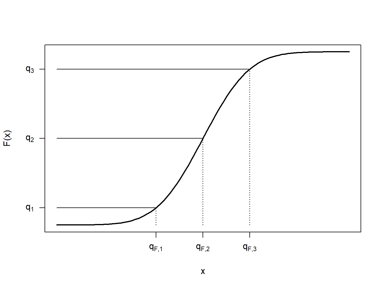
Figure 4.2: Continuous Quantile Case
Figure 4.3 shows three cases for distribution functions. The left panel corresponds to the continuous case just discussed. The middle panel displays a jump point similar to those we already saw in the empirical distribution function of Figure 4.1. For the value of \(q\) shown in this panel, we still have a unique value of the quantile \(q_F\). Even though there are many values of \(q\) such that \(F(q_F-) \le q \le F(q_F)\), for a particular value of \(q\), there is only one solution to equation (4.1). The right panel depicts a situation in which the quantile cannot be uniquely determined for the \(q\) shown as there is a range of \(q_F\)’s satisfying equation (4.1).
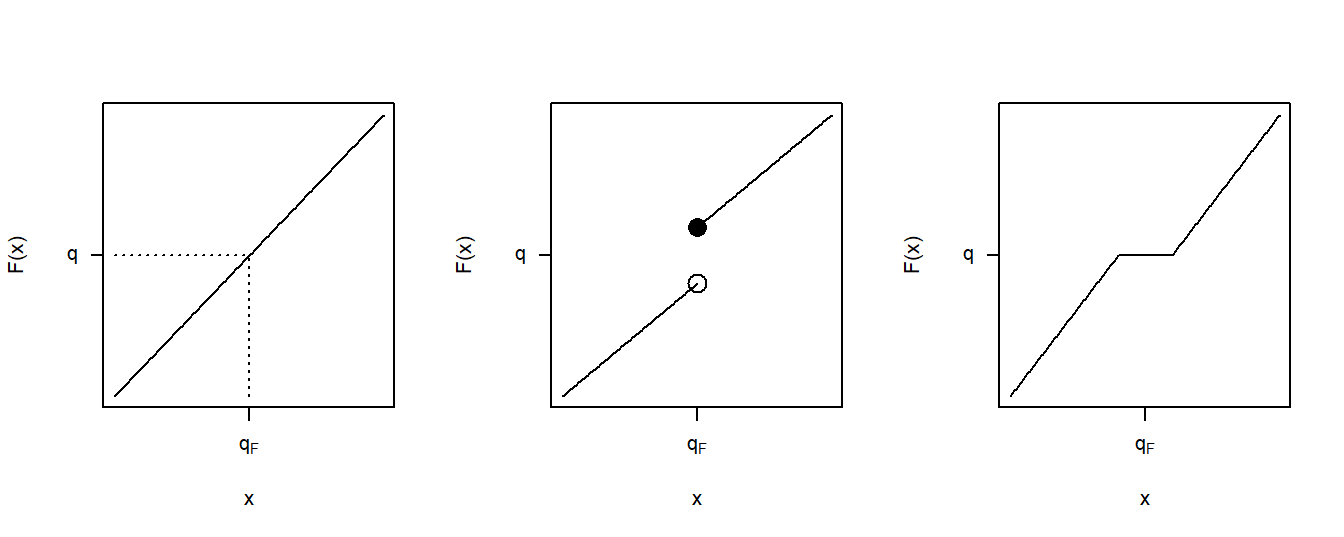
Figure 4.3: Three Quantile Cases
Example 4.1.2. Toy Data Set: Continued. Determine quantiles corresponding to the 20th, 50th, and 95th percentiles.
Show Example Solution
By taking a weighted average between data observations, smoothed empirical quantiles can handle cases such as the right panel in Figure 4.3. The \(q\)th smoothed empirical quantileA quantile obtained by linear interpolation between two empirical quantiles, i.e. data points. is defined as \[ \hat{\pi}_q = (1-h) X_{(j)} + h X_{(j+1)} \] where \(j=\lfloor(n+1)q\rfloor\), \(h=(n+1)q-j\), and \(X_{(1)}, \ldots, X_{(n)}\) are the ordered values (known as the order statistics) corresponding to \(X_1, \ldots, X_n\). (Recall that the brackets \(\lfloor \cdot\rfloor\) are the floor function denoting the greatest integer value.) Note that \(\hat{\pi}_q\) is simply a linear interpolation between \(X_{(j)}\) and \(X_{(j+1)}\).
Example 4.1.3. Toy Data Set: Continued. Determine the 50th and 20th smoothed percentiles.
Show Example Solution
4.1.1.4 Density Estimators
Discrete Variable. When the random variable is discrete, estimating the probability mass function \(f(x) = \Pr(X=x)\) is straightforward. We simply use the sample average, defined to be
\[ f_n(x) = \frac{1}{n} \sum_{i=1}^n I(X_i = x), \]
which is the proportion of the sample equal to \(x\).
Continuous Variable within a Group. For a continuous random variable, consider a discretized formulation in which the domain of \(F(\cdot)\) is partitioned by constants \(\{c_0 < c_1 < \cdots < c_k\}\) into intervals of the form \([c_{j-1}, c_j)\), for \(j=1, \ldots, k\). The data observations are thus “grouped” by the intervals into which they fall. Then, we might use the basic definition of the empirical mass function, or a variation such as \[f_n(x) = \frac{n_j}{n \times (c_j - c_{j-1})} \ \ \ \ \ \ c_{j-1} \le x < c_j,\] where \(n_j\) is the number of observations (\(X_i\)) that fall into the interval \([c_{j-1}, c_j)\).
Continuous Variable (not grouped). Extending this notion to instances where we observe individual data, note that we can always create arbitrary groupings and use this formula. More formally, let \(b>0\) be a small positive constant, known as a bandwidthA small positive constant that defines the width of the steps and the degree of smoothing., and define a density estimator to be
\[\begin{equation} f_n(x) = \frac{1}{2nb} \sum_{i=1}^n I(x-b < X_i \le x + b) \tag{4.2} \end{equation}\]
Show A Snippet of Theory
More generally, define the kernel density estimatorA nonparametric estimator of the density function of a random variable. of the pdfProbability density function at \(x\) as
\[\begin{equation} f_n(x) = \frac{1}{nb} \sum_{i=1}^n w\left(\frac{x-X_i}{b}\right) , \tag{4.3} \end{equation}\]
where \(w\) is a probability density function centered about 0. Note that equation (4.2) is a special case of the kernel density estimator where \(w(x) = \frac{1}{2}I(-1 < x \le 1)\), also known as the uniform kernel. Other popular choices are shown in Table 4.1.
Table 4.1. Popular Kernel Choices
\[ {\small \begin{matrix} \begin{array}{l|cc} \hline \text{Kernel} & w(x) \\ \hline \text{Uniform } & \frac{1}{2}I(-1 < x \le 1) \\ \text{Triangle} & (1-|x|)\times I(|x| \le 1) \\ \text{Epanechnikov} & \frac{3}{4}(1-x^2) \times I(|x| \le 1) \\ \text{Gaussian} & \phi(x) \\ \hline \end{array}\end{matrix} } \]
Here, \(\phi(\cdot)\) is the standard normal density function. As we will see in the following example, the choice of bandwidth \(b\) comes with a bias-variance tradeoffThe tradeoff between model simplicity (underfitting; high bias) and flexibility (overfitting; high variance). between matching local distributional features and reducing the volatility.
Example 4.1.4. Property Fund. Figure 4.4 shows a histogram (with shaded gray rectangles) of logarithmic property claims from 2010. The (blue) thick curve represents a Gaussian kernel density where the bandwidth was selected automatically using an ad hoc rule based on the sample size and volatility of these data. For this dataset, the bandwidth turned out to be \(b=0.3255\). For comparison, the (red) dashed curve represents the density estimator with a bandwidth equal to 0.1 and the green smooth curve uses a bandwidth of 1. As anticipated, the smaller bandwidth (0.1) indicates taking local averages over less data so that we get a better idea of the local average, but at the price of higher volatility. In contrast, the larger bandwidth (1) smooths out local fluctuations, yielding a smoother curve that may miss perturbations in the local average. For actuarial applications, we mainly use the kernel density estimator to get a quick visual impression of the data. From this perspective, you can simply use the default ad hoc rule for bandwidth selection, knowing that you have the ability to change it depending on the situation at hand.
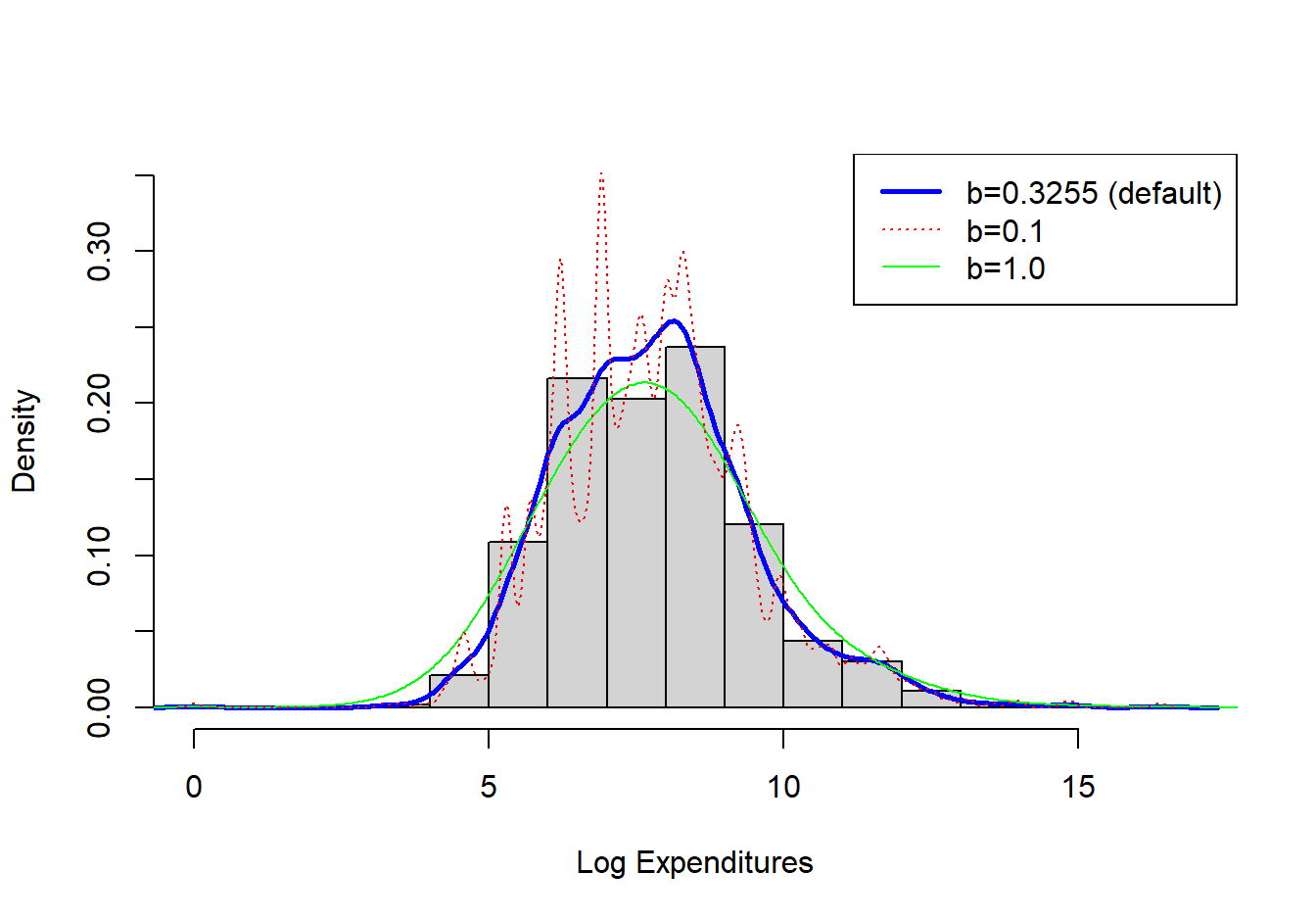
Figure 4.4: Histogram of Logarithmic Property Claims with Superimposed Kernel Density Estimators
Show R Code
Nonparametric density estimators, such as the kernel estimator, are regularly used in practice. The concept can also be extended to give smooth versions of an empirical distribution function. Given the definition of the kernel density estimator, the kernel estimator of the distribution function can be found as
\[ \begin{aligned} \tilde{F}_n(x) = \frac{1}{n} \sum_{i=1}^n W\left(\frac{x-X_i}{b}\right).\end{aligned} \]
where \(W\) is the distribution function associated with the kernel density \(w\). To illustrate, for the uniform kernel, we have \(w(y) = \frac{1}{2}I(-1 < y \le 1)\), so
\[ \begin{aligned} W(y) = \begin{cases} 0 & y<-1\\ \frac{y+1}{2}& -1 \le y < 1 \\ 1 & y \ge 1 \\ \end{cases}\end{aligned} . \]
Example 4.1.5. Actuarial Exam Question.
You study five lives to estimate the time from the onset of a disease to death. The times to death are:
\[ \begin{array}{ccccc} 2 & 3 & 3 & 3 & 7 \\ \end{array} \]
Using a triangular kernel with bandwidth \(2\), calculate the density function estimate at 2.5.
Show Example Solution
4.1.1.5 Plug-in Principle
One way to create a nonparametric estimator of some quantity is to use the analog or plug-in principleThe plug-in principle or analog principle of estimation proposes that population parameters be estimated by sample statistics which have the same property in the sample as the parameters do in the population. where one replaces the unknown cdfCumulative distribution function \(F\) with a known estimate such as the empirical cdf \(F_n\). So, if we are trying to estimate \(\mathrm{E}~[\mathrm{g}(X)]=\mathrm{E}_F~[\mathrm{g}(X)]\) for a generic function g, then we define a nonparametric estimator to be \(\mathrm{E}_{F_n}~[\mathrm{g}(X)]=n^{-1}\sum_{i=1}^n \mathrm{g}(X_i)\).
To see how this works, as a special case of g we consider the loss per payment random variable is \(Y = (X-d)_+\) and the loss elimination ratio introduced in Section 3.4.1. We can express this as \[ LER(d) = \frac{\mathrm{E~}[X - (X-d)_+]}{\mathrm{E~}[X]} =\frac{\mathrm{E~}[\min(X,d)]}{\mathrm{E~}[X]} , \] for a fixed deductible \(d\).
Example. 4.1.6. Bodily Injury Claims and Loss Elimination Ratios
We use a sample of 432 closed auto claims from Boston from Derrig, Ostaszewski, and Rempala (2001). Losses are recorded for payments due to bodily injuries in auto accidents. Losses are not subject to deductibles but are limited by various maximum coverage amounts that are also available in the data. It turns out that only 17 out of 432 (\(\approx\) 4%) were subject to these policy limits and so we ignore these data for this illustration.
The average loss paid is 6906 in U.S. dollars. Figure 4.5 shows other aspects of the distribution. Specifically, the left-hand panel shows the empirical distribution function, the right-hand panel gives a nonparametric density plot.
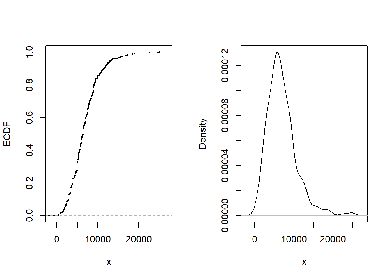
Figure 4.5: Bodily Injury Claims. The left-hand panel gives the empirical distribution function. The right-hand panel presents a nonparametric density plot.
The impact of bodily injury losses can be mitigated by the imposition of limits or purchasing reinsurance policies (see Section 10.3). To quantify the impact of these risk mitigation tools, it is common to compute the loss elimination ratio (LER) as introduced in Section 3.4.1. The distribution function is not available and so must be estimated in some way. Using the plug-in principle, a nonparametric estimator can be defined as
\[ LER_n(d) = \frac{n^{-1} \sum_{i=1}^n \min(X_i,d)}{n^{-1} \sum_{i=1}^n X_i} = \frac{\sum_{i=1}^n \min(X_i,d)}{\sum_{i=1}^n X_i} . \]
Figure 4.6 shows the estimator \(LER_n(d)\) for various choices of \(d\). For example, at \(d=1,000\), we have \(LER_n(1000) \approx\) 0.1442. Thus, imposing a limit of 1,000 means that expected retained claims are 14.42 percent lower when compared to expected claims with a zero deductible.
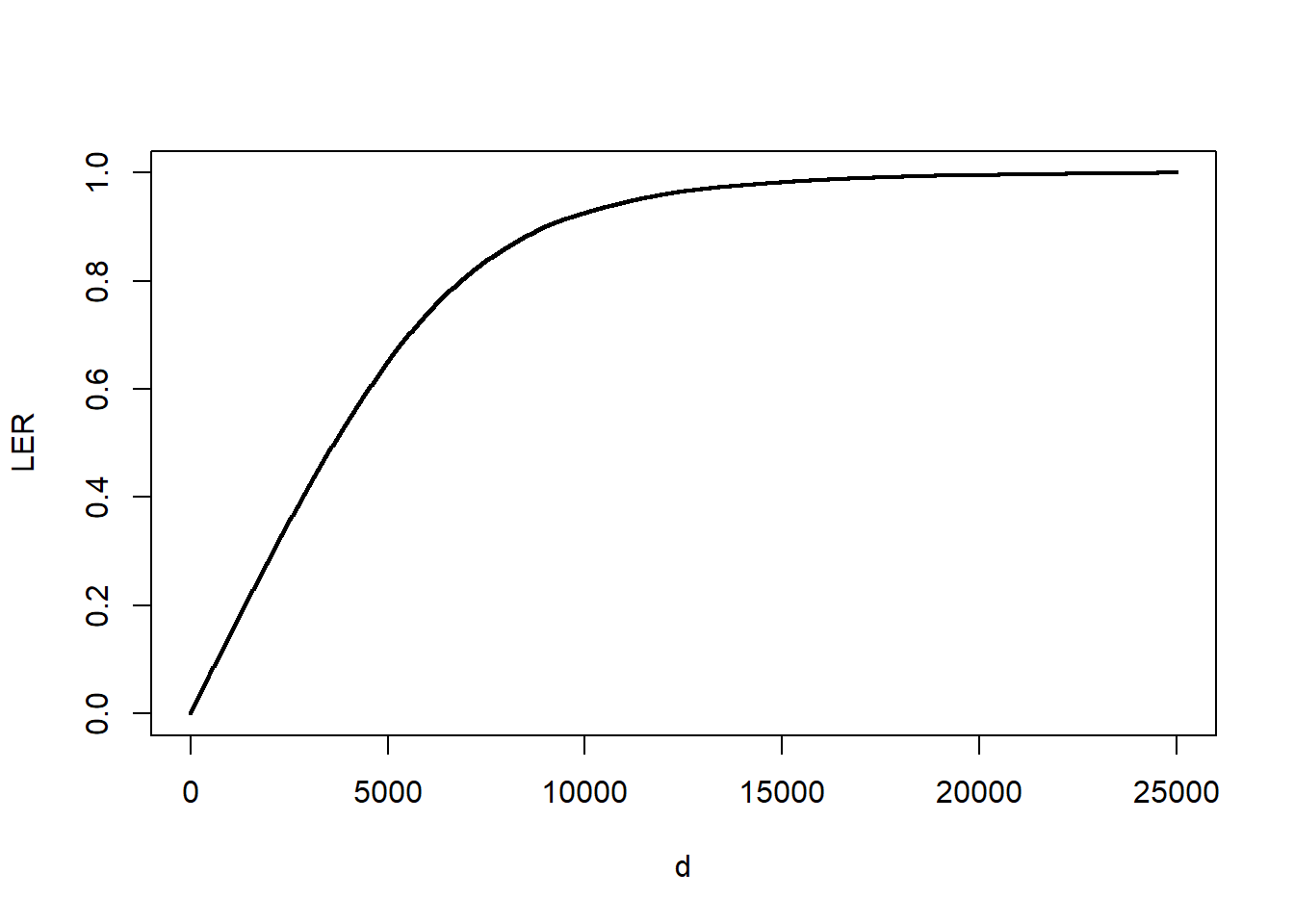
Figure 4.6: LER for Bodily Injury Claims. The figure presents the loss elimination ratio (LER) as a function of deductible \(d\).
4.1.2 Tools for Model Selection and Diagnostics
The previous section introduced nonparametric estimators in which there was no parametric form assumed about the underlying distributions. However, in many actuarial applications, analysts seek to employ a parametric fit of a distribution for ease of explanation and the ability to readily extend it to more complex situations such as including explanatory variables in a regression setting. When fitting a parametric distribution, one analyst might try to use a gamma distribution to represent a set of loss data. However, another analyst may prefer to use a Pareto distribution. How does one determine which model to select?
Nonparametric tools can be used to corroborate the selection of parametric models. Essentially, the approach is to compute selected summary measures under a fitted parametric model and to compare it to the corresponding quantity under the nonparametric model. As the nonparametric model does not assume a specific distribution and is merely a function of the data, it is used as a benchmark to assess how well the parametric distribution/model represents the data. Also, as the sample size increases, the empirical distribution converges almost surely to the underlying population distribution (by the strong law of large numbers). Thus the empirical distribution is a good proxy for the population. The comparison of parametric to nonparametric estimators may alert the analyst to deficiencies in the parametric model and sometimes point ways to improving the parametric specification. Procedures geared towards assessing the validity of a model are known as model diagnosticsProcedures to assess the validity of a model.
4.1.2.1 Graphical Comparison of Distributions
We have already seen the technique of overlaying graphs for comparison purposes. To reinforce the application of this technique, Figure 4.7 compares the empirical distribution to two parametric fitted distributions. The left panel shows the distribution functions of claims distributions. The dots forming an “S-shaped” curve represent the empirical distribution function at each observation. The thick blue curve gives corresponding values for the fitted gamma distribution and the light purple is for the fitted Pareto distribution. Because the Pareto is much closer to the empirical distribution function than the gamma, this provides evidence that the Pareto is the better model for this data set. The right panel gives similar information for the density function and provides a consistent message. Based (only) on these figures, the Pareto distribution is the clear choice for the analyst.
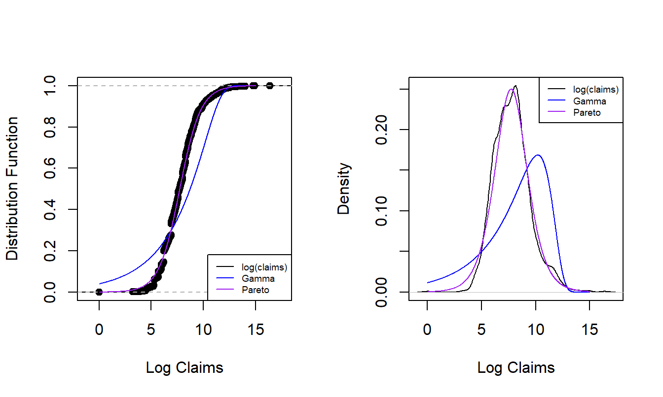
Figure 4.7: Nonparametric Versus Fitted Parametric Distribution and Density Functions. The left-hand panel compares distribution functions, with the dots corresponding to the empirical distribution, the thick blue curve corresponding to the fitted gamma and the light purple curve corresponding to the fitted Pareto. The right hand panel compares these three distributions summarized using probability density functions.
For another way to compare the appropriateness of two fitted models, consider the probability-probability (pp) plotA plot that compares two models through their cumulative probabilities.. A \(pp\) plot compares cumulative probabilities under two models. For our purposes, these two models are the nonparametric empirical distribution function and the parametric fitted model. Figure 4.8 shows \(pp\) plots for the Property Fund data introduced in Section 1.3. The fitted gamma is on the left and the fitted Pareto is on the right, compared to the same empirical distribution function of the data. The straight line represents equality between the two distributions being compared, so points close to the line are desirable. As seen in earlier demonstrations, the Pareto is much closer to the empirical distribution than the gamma, providing additional evidence that the Pareto is the better model.
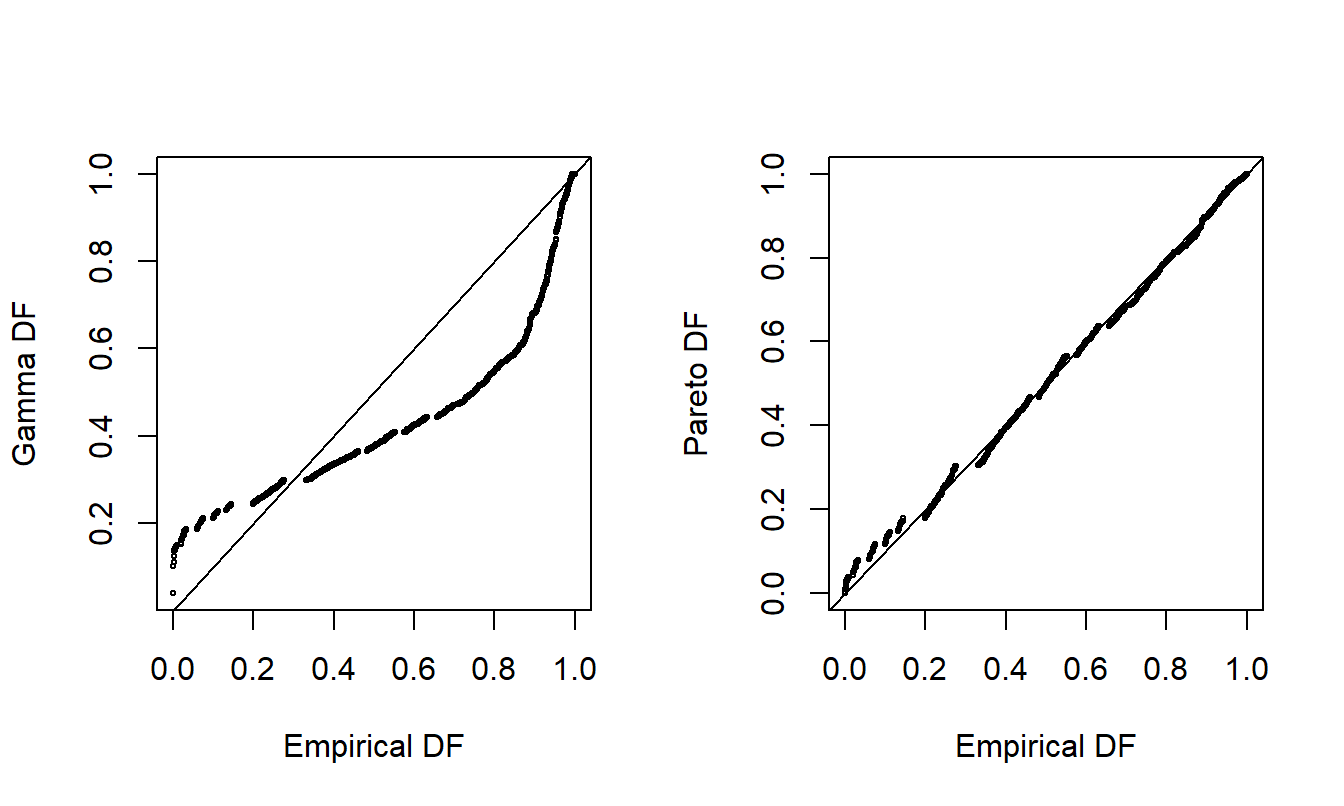
Figure 4.8: Probability-Probability (\(pp\)) Plots. The horizontal axis gives the empirical distribution function at each observation. In the left-hand panel, the corresponding distribution function for the gamma is shown in the vertical axis. The right-hand panel shows the fitted Pareto distribution. Lines of \(y=x\) are superimposed.
A \(pp\) plot is useful in part because no artificial scaling is required, such as with the overlaying of densities in Figure 4.7, in which we switched to the log scale to better visualize the data. The Chapter 4 Technical Supplement A.1 introduces a variation of the \(pp\) plot known as a Lorenz curveA graph of the proportion of a population on the horizontal axis and a distribution function of interest on the vertical axis.; this is an important tool for assessing income inequality. Furthermore, \(pp\) plots are available in multivariate settings where more than one outcome variable is available. However, a limitation of the \(pp\) plot is that, because it plots cumulative distribution functions, it can sometimes be difficult to detect where a fitted parametric distribution is deficient. As an alternative, it is common to use a quantile-quantile (qq) plotA plot that compares two models through their quantiles., as demonstrated in Figure 4.9.
The \(qq\) plot compares two fitted models through their quantiles. As with \(pp\) plots, we compare the nonparametric to a parametric fitted model. Quantiles may be evaluated at each point of the data set, or on a grid (e.g., at \(0, 0.001, 0.002, \ldots, 0.999, 1.000\)), depending on the application. In Figure 4.9, for each point on the aforementioned grid, the horizontal axis displays the empirical quantile and the vertical axis displays the corresponding fitted parametric quantile (gamma for the upper two panels, Pareto for the lower two). Quantiles are plotted on the original scale in the left panels and on the log scale in the right panels to allow us to see where a fitted distribution is deficient. The straight line represents equality between the empirical distribution and fitted distribution. From these plots, we again see that the Pareto is an overall better fit than the gamma. Furthermore, the lower-right panel suggests that the Pareto distribution does a good job with large claims, but provides a poorer fit for small claims.
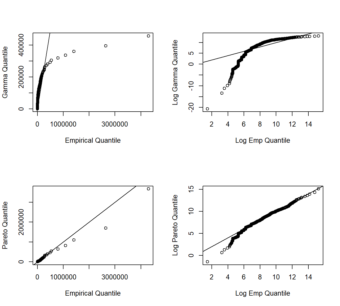
Figure 4.9: Quantile-Quantile (\(qq\)) Plots. The horizontal axis gives the empirical quantiles at each observation. The right-hand panels they are graphed on a logarithmic basis. The vertical axis gives the quantiles from the fitted distributions; gamma quantiles are in the upper panels, Pareto quantiles are in the lower panels.
Example 4.1.7. Actuarial Exam Question. The graph below shows a \(pp\) plot of a fitted distribution compared to a sample.
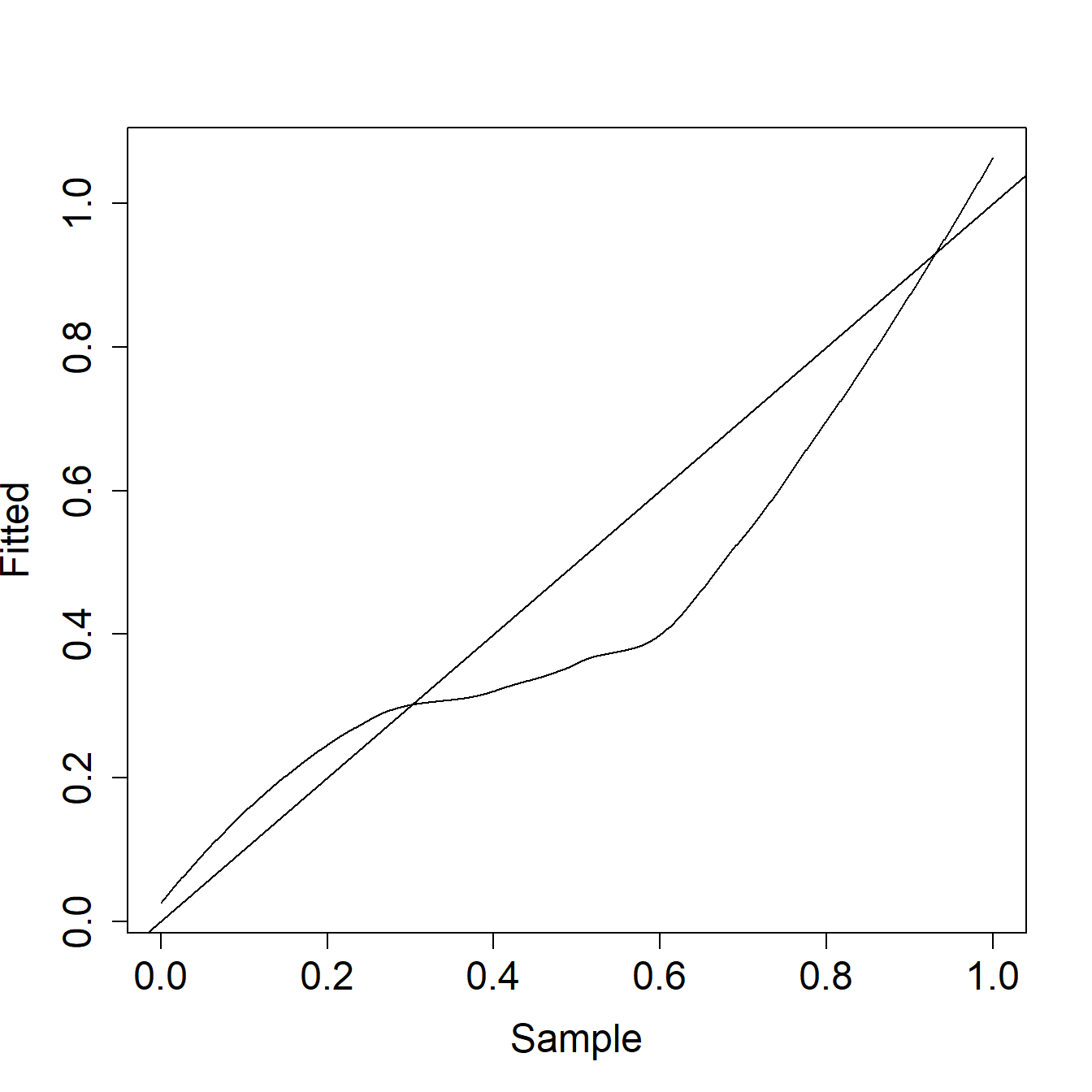
Comment on the two distributions with respect to left tail, right tail, and median probabilities.
Show Example Solution
4.1.2.2 Statistical Comparison of Distributions
When selecting a model, it is helpful to make the graphical displays presented. However, for reporting results, it can be effective to supplement the graphical displays with selected statistics that summarize model goodness of fit. Table 4.2 provides three commonly used goodness of fit statisticsA measure used to assess how well a statistical model fits the data, usually by summarizing the discrepancy between the observations and the expected values under the model.. In this table, \(F_n\) is the empirical distribution, \(F\) is the fitted or hypothesized distribution, and \(F_i^* = F(x_i)\).
Table 4.2. Three Goodness of Fit Statistics
\[ {\small \begin{matrix} \begin{array}{l|cc} \hline \text{Statistic} & \text{Definition} & \text{Computational Expression} \\ \hline \text{Kolmogorov-} & \max_x |F_n(x) - F(x)| & \max(D^+, D^-) \text{ where } \\ ~~~\text{Smirnov} && D^+ = \max_{i=1, \ldots, n} \left|\frac{i}{n} - F_i^*\right| \\ && D^- = \max_{i=1, \ldots, n} \left| F_i^* - \frac{i-1}{n} \right| \\ \text{Cramer-von Mises} & n \int (F_n(x) - F(x))^2 f(x) dx & \frac{1}{12n} + \sum_{i=1}^n \left(F_i^* - (2i-1)/n\right)^2 \\ \text{Anderson-Darling} & n \int \frac{(F_n(x) - F(x))^2}{F(x)(1-F(x))} f(x) dx & -n-\frac{1}{n} \sum_{i=1}^n (2i-1) \log\left(F_i^*(1-F_{n+1-i})\right)^2 \\ \hline \end{array} \\ \end{matrix} } \]
The Kolmogorov-Smirnov statistic is the maximum absolute difference between the fitted distribution function and the empirical distribution function. Instead of comparing differences between single points, the Cramer-von Mises statistic integrates the difference between the empirical and fitted distribution functions over the entire range of values. The Anderson-Darling statistic also integrates this difference over the range of values, although weighted by the inverse of the variance. It therefore places greater emphasis on the tails of the distribution (i.e when \(F(x)\) or \(1-F(x)=S(x)\) is small).
Example 4.1.8. Actuarial Exam Question (modified). A sample of claim payments is:
\[ \begin{array}{ccccc} 29 & 64 & 90 & 135 & 182 \\ \end{array} \]
Compare the empirical claims distribution to an exponential distribution with mean \(100\) by calculating the value of the Kolmogorov-Smirnov test statistic.
Show Example Solution
4.1.3 Starting Values
The method of moments and percentile matching are nonparametric estimation methods that provide alternatives to maximum likelihood. Generally, maximum likelihood is the preferred technique because it employs data more efficiently. (See Appendix Chapter 17 for precise definitions of efficiency.) However, methods of moments and percentile matching are useful because they are easier to interpret and therefore allow the actuary or analyst to explain procedures to others. Additionally, the numerical estimation procedure (e.g. if performed in R) for the maximum likelihood is iterative and requires starting values to begin the recursive process. Although many problems are robust to the choice of the starting values, for some complex situations, it can be important to have a starting value that is close to the (unknown) optimal value. Method of moments and percentile matching are techniques that can produce desirable estimates without a serious computational investment and can thus be used as a starting value for computing maximum likelihood.
4.1.3.1 Method of Moments
Under the method of momentsThe estimation of population parameters by approximating parametric moments using empirical sample moments., we approximate the moments of the parametric distribution using the empirical (nonparametric) moments described in Section 4.1.1.1. We can then algebraically solve for the parameter estimates.
Example 4.1.9. Property Fund. For the 2010 property fund, there are \(n=1,377\) individual claims (in thousands of dollars) with
\[m_1 = \frac{1}{n} \sum_{i=1}^n X_i = 26.62259 \ \ \ \ \text{and} \ \ \ \ m_2 = \frac{1}{n} \sum_{i=1}^n X_i^2 = 136154.6 .\] Fit the parameters of the gamma and Pareto distributions using the method of moments.
Show Example Solution
As the above example suggests, there is flexibility with the method of moments. For example, we could have matched the second and third moments instead of the first and second, yielding different estimators. Furthermore, there is no guarantee that a solution will exist for each problem. For data that are censored or truncated, matching moments is possible for a few problems but, in general, this is a more difficult scenario. Finally, for distributions where the moments do not exist or are infinite, method of moments is not available. As an alternative, one can use the percentile matching technique.
4.1.3.2 Percentile Matching
Under percentile matchingThe estimation of population parameters by approximating parametric percentiles using empirical quantiles., we approximate the quantiles or percentiles of the parametric distribution using the empirical (nonparametric) quantiles or percentiles described in Section 4.1.1.3.
Example 4.1.10. Property Fund. For the 2010 property fund, we illustrate matching on quantiles. In particular, the Pareto distribution is intuitively pleasing because of the closed-form solution for the quantiles. Recall that the distribution function for the Pareto distribution is \[F(x) = 1 - \left(\frac{\theta}{x+\theta}\right)^{\alpha}.\] Easy algebra shows that we can express the quantile as
\[F^{-1}(q) = \theta \left( (1-q)^{-1/\alpha} -1 \right).\] for a fraction \(q\), \(0<q<1\).
Determine estimates of the Pareto distribution parameters using the 25th and 95th empirical quantiles.
Show Example Solution
Example 4.1.11. Actuarial Exam Question. You are given:
- Losses follow a loglogistic distribution with cumulative distribution function: \[F(x) = \frac{\left(x/\theta\right)^{\gamma}}{1+\left(x/\theta\right)^{\gamma}}\]
- The sample of losses is:
\[ \begin{array}{ccccccccccc} 10 &35 &80 &86 &90 &120 &158 &180 &200 &210 &1500 \\ \end{array} \]
Calculate the estimate of \(\theta\) by percentile matching, using the 40th and 80th empirically smoothed percentile estimates.
Show Example Solution
Like the method of moments, percentile matching is almost too flexible in the sense that estimators can vary depending on different percentiles chosen. For example, one actuary may use estimation on the 25th and 95th percentiles whereas another uses the 20th and 80th percentiles. In general estimated parameters will differ and there is no compelling reason to prefer one over the other. Also as with the method of moments, percentile matching is appealing because it provides a technique that can be readily applied in selected situations and has an intuitive basis. Although most actuarial applications use maximum likelihood estimators, it can be convenient to have alternative approaches such as method of moments and percentile matching available.
Show Quiz Solution
4.2 Model Selection
In this section, you learn how to:
- Describe the iterative model selection specification process
- Outline steps needed to select a parametric model
- Describe pitfalls of model selection based purely on in-sample data when compared to the advantages of out-of-sample model validation
This section underscores the idea that model selection is an iterative process in which models are cyclically (re)formulated and tested for appropriateness before using them for inference. After an overview, we describe the model selectionThe process of selecting a statistical model from a set of candidate models using data. process based on:
- an in-sampleA dataset used for analysis and model development. also known as a training dataset. or training dataset,
- an out-of-sampleA dataset used for model validation. also known as a test dataset. or test dataset, and
- a method that combines these approaches known as cross-validationA model validation procedure in which the data sample is partitioned into subsamples, where splits are formed by separately taking each subsample as the out-of-sample dataset..
4.2.1 Iterative Model Selection
In our development, we examine the data graphically, hypothesize a model structure, and compare the data to a candidate model in order to formulate an improved model. Box (1980) describes this as an iterative process which is shown in Figure 4.10.
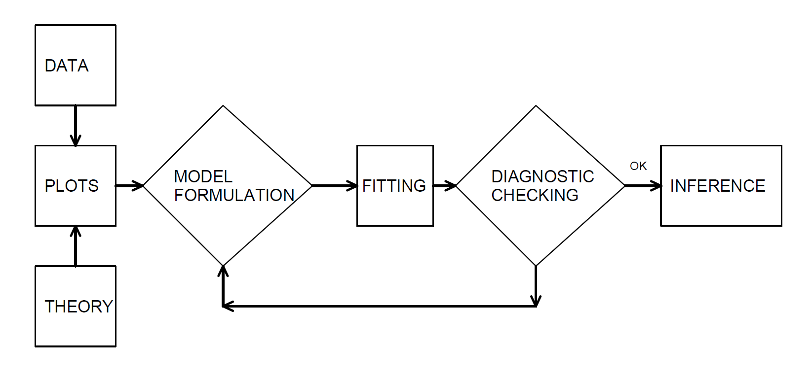
Figure 4.10: Iterative Model Specification Process
This iterative process provides a useful recipe for structuring the task of specifying a model to represent a set of data.
- The first step, the model formulation stage, is accomplished by examining the data graphically and using prior knowledge of relationships, such as from economic theory or industry practice.
- The second step in the iteration is fitting based on the assumptions of the specified model. These assumptions must be consistent with the data to make valid use of the model.
- The third step is diagnostic checking; the data and model must be consistent with one another before additional inferences can be made. Diagnostic checking is an important part of the model formulation; it can reveal mistakes made in previous steps and provide ways to correct these mistakes.
The iterative process also emphasizes the skills you need to make analytics work. First, you need a willingness to summarize information numerically and portray this information graphically. Second, it is important to develop an understanding of model properties. You should understand how a probabilistic model behaves in order to match a set of data to it. Third, theoretical properties of the model are also important for inferring general relationships based on the behavior of the data.
4.2.2 Model Selection Based on a Training Dataset
It is common to refer to a dataset used for analysis as an in-sample or training dataset. Techniques available for selecting a model depend upon whether the outcomes \(X\) are discrete, continuous, or a hybrid of the two, although the principles are the same.
Graphical and other Basic Summary Measures. Begin by summarizing the data graphically and with statistics that do not rely on a specific parametric form, as summarized in Section 4.1. Specifically, you will want to graph both the empirical distribution and density functions. Particularly for loss data that contain many zeros and that can be skewed, deciding on the appropriate scale (e.g., logarithmic) may present some difficulties. For discrete data, tables are often preferred. Determine sample moments, such as the mean and variance, as well as selected quantiles, including the minimum, maximum, and the median. For discrete data, the mode (or most frequently occurring value) is usually helpful.
These summaries, as well as your familiarity of industry practice, will suggest one or more candidate parametric models. Generally, start with the simpler parametric models (for example, one parameter exponential before a two parameter gamma), gradually introducing more complexity into the modeling process.
Critique the candidate parametric model numerically and graphically. For the graphs, utilize the tools introduced in Section 4.1.2 such as \(pp\) and \(qq\) plots. For the numerical assessments, examine the statistical significance of parameters and try to eliminate parameters that do not provide additional information.
Likelihood Ratio Tests. For comparing model fits, if one model is a subset of another, then a likelihood ratio test may be employed; the general approach to likelihood ratio testing is described in Sections 15.4.3 and 17.3.2.
Goodness of Fit Statistics. Generally, models are not proper subsets of one another so overall goodness of fit statistics are helpful for comparing models. Information criteria are one type of goodness of statistic. The most widely used examples are Akaike’s Information Criterion (AIC) and the (Schwarz) Bayesian Information Criterion (BIC); they are widely cited because they can be readily generalized to multivariate settings. Section 15.4.4 provides a summary of these statistics.
For selecting the appropriate distribution, statistics that compare a parametric fit to a nonparametric alternative, summarized in Section 4.1.2.2, are useful for model comparison. For discrete data, a goodness of fit statistic (as described in Section 2.7) is generally preferred as it is more intuitive and simpler to explain.
4.2.3 Model Selection Based on a Test Dataset
Model validationThe process of confirming that the proposed model is appropriate. is the process of confirming that the proposed model is appropriate, especially in light of the purposes of the investigation. An important limitation of the model selection process based only on in-sample data is that it can be susceptible to data-snoopingRepeatedly fitting models to a data set without a prior hypothesis of interest., that is, fitting a great number of models to a single set of data. By looking at a large number of models, we may overfit the data and understate the natural variation in our representation.
Selecting a model based only on in-sample data also does not support the goal of predictive inferencePreditive inference is the process of using past data observations to predict future observations.. Particularly in actuarial applications, our goal is to make statements about new experience rather than a dataset at hand. For example, we use claims experience from one year to develop a model that can be used to price insurance contracts for the following year. As an analogy, we can think about the training data set as experience from one year that is used to predict the behavior of the next year’s test data set.
We can respond to these criticisms by using a technique known as out-of-sample validation. The ideal situation is to have available two sets of data, one for training, or model development, and the other for testing, or model validation. We initially develop one or several models on the first data set that we call our candidate models. Then, the relative performance of the candidate models can be measured on the second set of data. In this way, the data used to validate the model are unaffected by the procedures used to formulate the model.
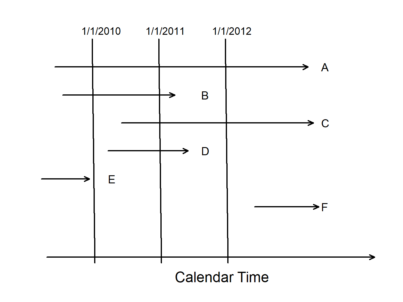
Random Split of the Data. Unfortunately, rarely will two sets of data be available to the investigator. However, we can implement the validation process by splitting the data set into training and test subsamples, respectively. Figure 4.11 illustrates this splitting of the data.
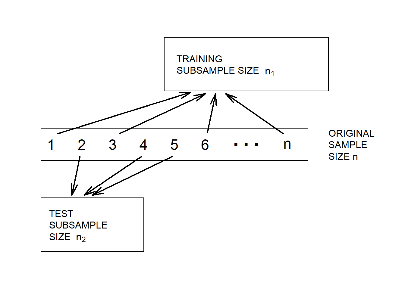
Figure 4.11: Model Validation. A data set is randomly split into two subsamples.
Various researchers recommend different proportions for the allocation. Snee (1977) suggests that data-splitting not be done unless the sample size is moderately large. The guidelines of Picard and Berk (1990) show that the greater the number of parameters to be estimated, the greater the proportion of observations needed for the model development subsample.
Model Validation Statistics. Much of the literature supporting the establishment of a model validation process is based on regression and classification models that you can think of as an input-output problem (James et al. (2013)). That is, we have several inputs \(x_1, \ldots, x_k\) that are related to an output \(y\) through a function such as \[y = \mathrm{g}\left(x_1, \ldots, x_k\right).\] One uses the training sample to develop an estimate of \(\mathrm{g}\), say, \(\hat{\mathrm{g}}\), and then calibrate the distance from the observed outcomes to the predictions using a criterion of the form
\[\begin{equation} \sum_i \mathrm{d}(y_i,\hat{\mathrm{g}}\left(x_{i1}, \ldots, x_{ik}\right) ) . \tag{4.4} \end{equation}\]
Here, “d” is some measure of distance and the sum \(i\) is over the test data. In many regression applications, it is common to use squared Euclidean distance of the form \(\mathrm{d}(y_i,\mathrm{g}) = (y_i-\mathrm{g})^2\). In actuarial applications, Euclidean distance \(\mathrm{d}(y_i,\mathrm{g}) = |y_i-\mathrm{g}|\) is often preferred because of the skewed nature of the data (large outlying values of \(y\) can have a large effect on the measure). Chapter 7 describes another measure, the Gini indexA measure for assessing income inequality. it measures the discrepancy between the income and population distributions and is calculated from the lorenz curve., that is useful in actuarial applications particularly when there is a large proportion of zeros in claims data (corresponding to no claims).
Selecting a Distribution. Still, our focus so far has been to select a distribution for a data set that can be used for actuarial modeling without additional inputs \(x_1, \ldots, x_k\). Even in this more fundamental problem, the model validation approach is valuable. If we base all inference on only in-sample data, then there is a tendency to select more complicated models than needed. For example, we might select a four parameter GB2, generalized beta of the second kind, distribution when only a two parameter Pareto is needed. Information criteria such as AICAkaike’s information criterion and BICBayesian information criterion included penalties for model complexity and so provide some protection but using a test sample is the best guarantee to achieve parsimonious models. From a quote often attributed to Albert Einstein, we want to “use the simplest model as possible but no simpler.”
4.2.4 Model Selection Based on Cross-Validation
Although out-of-sample validation is the gold standard in predictive modeling, it is not always practical to do so. The main reason is that we have limited sample sizes and the out-of-sample model selection criterion in equation (4.4) depends on a random split of the data. This means that different analysts, even when working the same data set and same approach to modeling, may select different models. This is likely in actuarial applications because we work with skewed data sets where there is a large chance of getting some very large outcomes and large outcomes may have a great influence on the parameter estimates.
Cross-Validation Procedure. Alternatively, one may use cross-validation, as follows.
- The procedure begins by using a random mechanism to split the data into \(K\) subsets of roughly equal size known as folds, where analysts typically use 5 to 10.
- Next, one uses the first \(K\)-1 subsamples to estimate model parameters. Then, “predict” the outcomes for the \(K\)th subsample and use a measure such as in equation (4.4) to summarize the fit.
- Now, repeat this by holding out each of the \(K\) subsamples, summarizing with an out-of-sample statistic. Thus, summarize these \(K\) statistics, typically by averaging, to give a single overall statistic for comparison purposes.
Repeat these steps for several candidate models and choose the model with the lowest overall cross-validation statistic.
Cross-validation is widely used because it retains the predictive flavor of the out-of-sample model validation process but, due to the re-use of the data, is more stable over random samples.
Show Quiz Solution
4.3 Estimation using Modified Data
In this section, you learn how to:
- Describe grouped, censored, and truncated data
- Estimate parametric distributions based on grouped, censored, and truncated data
- Estimate distributions nonparametrically based on grouped, censored, and truncated data
4.3.1 Parametric Estimation using Modified Data
Basic theory and many applications are based on individual observations that are “complete” and “unmodified,” as we have seen in the previous section. Section 3.5 introduced the concept of observations that are “modified” due to two common types of limitations: censoring and truncation. For example, it is common to think about an insurance deductible as producing data that are truncated (from the left) or policy limits as yielding data that are censored (from the right). This viewpoint is from the primary insurer (the seller of the insurance). Another viewpoint is that of a reinsurer (an insurer of an insurance company) that will be discussed more in Chapter 10. A reinsurer may not observe a claim smaller than an amount, only that a claim exists; this is an example of censoring from the left. So, in this section, we cover the full gamut of alternatives. Specifically, this section will address parametric estimation methods for three alternatives to individual, complete, and unmodified data: interval-censored data available only in groups, data that are limited or censored, and data that may not be observed due to truncation.
4.3.1.1 Parametric Estimation using Grouped Data
Consider a sample of size \(n\) observed from the distribution \(F(\cdot)\), but in groups so that we only know the group into which each observation fell, not the exact value. This is referred to as grouped or interval-censored data. For example, we may be looking at two successive years of annual employee records. People employed in the first year but not the second have left sometime during the year. With an exact departure date (individual data), we could compute the amount of time that they were with the firm. Without the departure date (grouped data), we only know that they departed sometime during a year-long interval.
Formalizing this idea, suppose there are \(k\) groups or intervals delimited by boundaries \(c_0 < c_1< \cdots < c_k\). For each observation, we only observe the interval into which it fell (e.g. \((c_{j-1}, c_j)\)), not the exact value. Thus, we only know the number of observations in each interval. The constants \(\{c_0 < c_1 < \cdots < c_k\}\) form some partition of the domain of \(F(\cdot)\). Then the probability of an observation \(X_i\) falling in the \(j\)th interval is \[\Pr\left(X _i \in (c_{j-1}, c_j]\right) = F(c_j) - F(c_{j-1}).\]
The corresponding probability mass function for an observation is
\[ \begin{aligned} f(x) &= \begin{cases} F(c_1) - F(c_{0}) & \text{if }\ x \in (c_{0}, c_1]\\ \vdots & \vdots \\ F(c_k) - F(c_{k-1}) & \text{if }\ x \in (c_{k-1}, c_k]\\ \end{cases} \\ &= \prod_{j=1}^k \left\{F(c_j) - F(c_{j-1})\right\}^{I(x \in (c_{j-1}, c_j])} \end{aligned} \]
Now, define \(n_j\) to be the number of observations that fall in the \(j\)th interval, \((c_{j-1}, c_j]\). Thus, the likelihood functionA function of the likeliness of the parameters in a model, given the observed data. (with respect to the parameter(s) \(\theta\)) is
\[ \begin{aligned} L(\theta) = \prod_{j=1}^n f(x_i) = \prod_{j=1}^k \left\{F(c_j) - F(c_{j-1})\right\}^{n_j} \end{aligned} \]
And the log-likelihood function is \[ \begin{aligned} l(\theta) = \log L(\theta) = \log \prod_{j=1}^n f(x_i) = \sum_{j=1}^k n_j \log \left\{F(c_j) - F(c_{j-1})\right\} \end{aligned} \]
Maximizing the likelihood function (or equivalently, maximizing the log-likelihood function) would then produce the maximum likelihood estimates for grouped data.
Example 4.3.1. Actuarial Exam Question. You are given:
- Losses follow an exponential distribution with mean \(\theta\).
- A random sample of 20 losses is distributed as follows:
\[ {\small \begin{array}{l|c} \hline \text{Loss Range} & \text{Frequency} \\ \hline [0,1000] & 7 \\ (1000,2000] & 6 \\ (2000,\infty) & 7 \\ \hline \end{array} } \]
Calculate the maximum likelihood estimate of \(\theta\).
Show Example Solution
4.3.1.2 Censored Data
Censoring occurs when we record only a limited value of an observation. The most common form is right-censoring, in which we record the smaller of the “true” dependent variable and a censoring value. Using notation, let \(X\) represent an outcome of interest, such as the loss due to an insured event or time until an event. Let \(C_U\) denote the censoring amount. With right-censored observations, we record \(X_U^{\ast}= \min(X, C_U) = X \wedge C_U\). We also record whether or not censoring has occurred. Let \(\delta_U= I(X \le C_U)\) be a binary variable that is 0 if censoring occurs and 1 if it does not, that is, \(\delta_U\) indicates whether or not \(X\) is uncensored.
For an example that we saw in Section 3.4.2, \(C_U\) may represent the upper limit of coverage of an insurance policy (we used \(u\) for the upper limit in that section). The loss may exceed the amount \(C_U\), but the insurer only has \(C_U\) in its records as the amount paid out and does not have the amount of the actual loss \(X\) in its records.
Similarly, with left-censoring, we record the larger of a variable of interest and a censoring variable. If \(C_L\) is used to represent the censoring amount, we record \(X_L^{\ast}= \max(X, C_L)\) along with the censoring indicator \(\delta_L= I(X > C_L)\).
As an example, you got a brief introduction to reinsurance (insurance for insurers) in Section 3.4.4 and will see more in Chapter 10. Suppose a reinsurer will cover insurer losses greater than \(C_L\); this means that the reinsurer is responsible for the excess of \(X_L^{\ast}\) over \(C_L\). Using notation, the loss of the reinsurer is \(Y = X_L^{\ast} - C_L\). To see this, first consider the case where the policyholder loss \(X < C_L\). Then, the insurer will pay the entire claim and \(Y =C_L- C_L=0\), no loss for the reinsurer. For contrast, if the loss \(X \ge C_L\), then \(Y = X-C_L\) represents the reinsurer’s retained claims. Put another way, if a loss occurs, the reinsurer records the actual amount if it exceeds the limit \(C_L\) and otherwise it only records that it had a loss of \(0\).
4.3.1.3 Truncated Data
Censored observations are recorded for study, although in a limited form. In contrast, truncated outcomes are a type of missing data. An outcome is potentially truncated when the availability of an observation depends on the outcome.
In insurance, it is common for observations to be left-truncated at \(C_L\) when the amount is \[ \begin{aligned} Y &= \left\{ \begin{array}{cl} \text{we do not observe }X & X \le C_L \\ X & X > C_L \end{array} \right.\end{aligned} . \]
In other words, if \(X\) is less than the threshold \(C_L\), then it is not observed.
For an example we saw in Section 3.4.1, \(C_L\) may represent the deductible of an insurance policy (we used \(d\) for the deductible in that section). If the insured loss is less than the deductible, then the insurer may not observe or record the loss at all. If the loss exceeds the deductible, then the excess \(X-C_L\) is the claim that the insurer covers. In Section 3.4.1, we defined the per payment loss to be \[ Y^{P} = \left\{ \begin{matrix} \text{Undefined} & X \le d \\ X - d & X > d \end{matrix} \right. , \] so that if a loss exceeds a deductible, we record the excess amount \(X-d\). This is very important when considering amounts that the insurer will pay. However, for estimation purposes of this section, it matters little if we subtract a known constant such as \(C_L=d\). So, for our truncated variable \(Y\), we use the simpler convention and do not subtract \(d\).
Similarly for right-truncated data, if \(X\) exceeds a threshold \(C_U\), then it is not observed. In this case, the amount is \[ \begin{aligned} Y &= \left\{ \begin{array}{cl} X & X \le C_U \\ \text{we do not observe }X & X > C_U. \end{array} \right.\end{aligned} \]
Classic examples of truncation from the right include \(X\) as a measure of distance to a star. When the distance exceeds a certain level \(C_U\), the star is no longer observable.
Figure 4.12 compares truncated and censored observations. Values of \(X\) that are greater than the “upper” censoring limit \(C_U\) are not observed at all (right-censored), while values of \(X\) that are smaller than the “lower” truncation limit \(C_L\) are observed, but observed as \(C_L\) rather than the actual value of \(X\) (left-truncated).
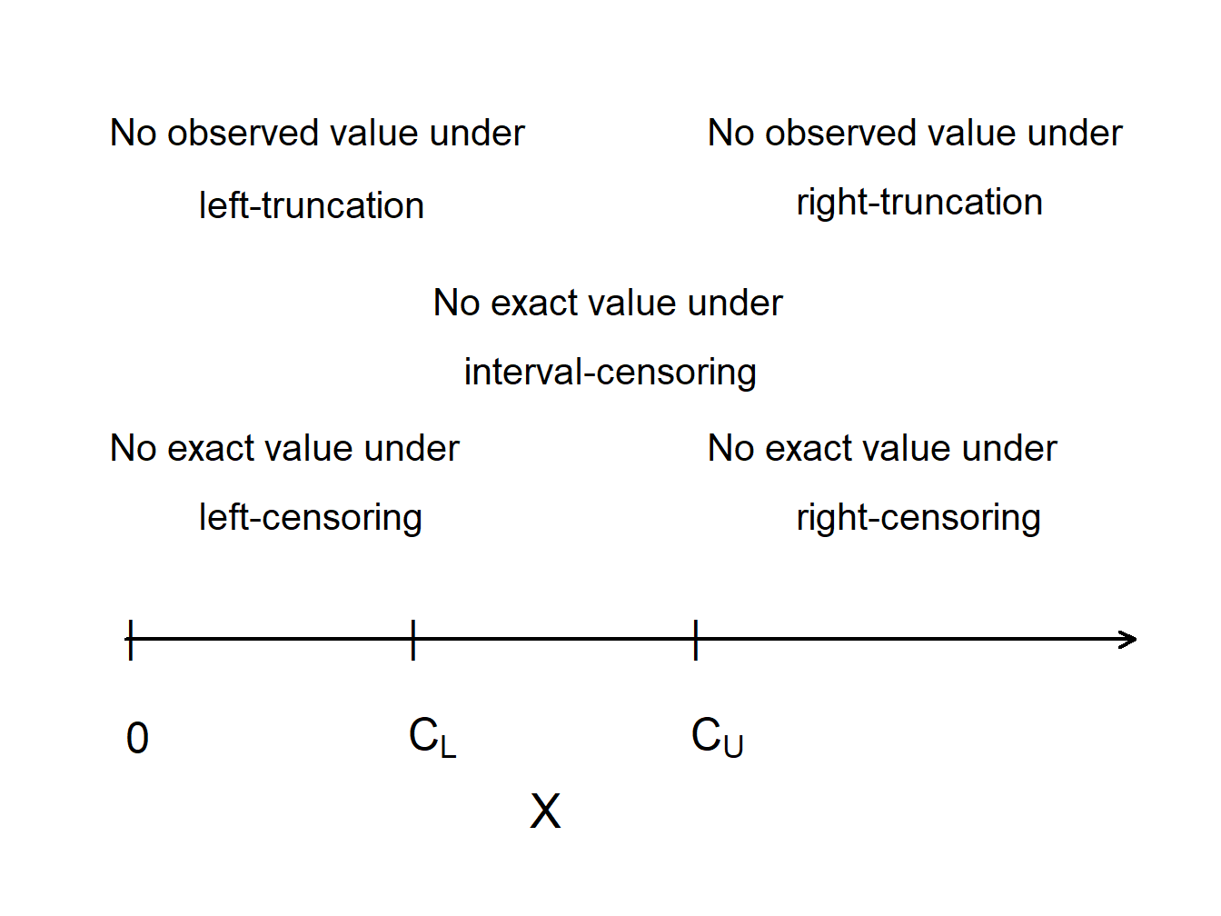
Figure 4.12: Censoring and Truncation
Show Mortality Study Example
To summarize, for outcome \(X\) and constants \(C_L\) and \(C_U\),
| Limitation Type | Limited Variable | Recording Information |
|---|---|---|
| right censoring | \(X_U^{\ast}= \min(X, C_U)\) | \(\delta_U= I(X \le C_U)\) |
| left censoring | \(X_L^{\ast}= \max(X, C_L)\) | \(\delta_L= I(X > C_L)\) |
| interval censoring | ||
| right truncation | \(X\) | observe \(X\) if \(X \le C_U\) |
| left truncation | \(X\) | observe \(X\) if \(X > C_L\) |
4.3.1.4 Parametric Estimation using Censored and Truncated Data
For simplicity, we assume non-random censoring amounts and a continuous outcome \(X\). To begin, consider the case of right-censored data where we record \(X_U^{\ast}= \min(X, C_U)\) and censoring indicator \(\delta= I(X \le C_U)\). If censoring occurs so that \(\delta=0\), then \(X > C_U\) and the likelihood is \(\Pr(X > C_U) = 1-F(C_U)\). If censoring does not occur so that \(\delta=1\), then \(X \le C_U\) and the likelihood is \(f(x)\). Summarizing, we have the likelihood of a single observation as
\[ \begin{aligned} \left\{ \begin{array}{ll} 1-F(C_U) & \text{if }\delta=0 \\ f(x) & \text{if } \delta = 1 \end{array} \right. = \left\{ f(x)\right\}^{\delta} \left\{1-F(C_U)\right\}^{1-\delta} . \end{aligned} \]
The right-hand expression allows us to present the likelihood more compactly. Now, for an iid sample of size \(n\), the likelihood is
\[ L(\theta) = \prod_{i=1}^n \left\{ f(x_i)\right\}^{\delta_i} \left\{1-F(C_{Ui})\right\}^{1-\delta_i} = \prod_{\delta_i=1} f(x_i) \prod_{\delta_i=0} \{1-F(C_{Ui})\}, \]
with potential censoring times \(\{ C_{U1}, \ldots,C_{Un} \}\). Here, the notation “\(\prod_{\delta_i=1}\)” means to take the product over uncensored observations, and similarly for “\(\prod_{\delta_i=0}\).”
On the other hand, truncated data are handled in likelihood inference via conditional probabilities. Specifically, we adjust the likelihood contribution by dividing by the probability that the variable was observed. To summarize, we have the following contributions to the likelihood function for six types of outcomes:
\[ {\small \begin{array}{lc} \hline \text{Outcome} & \text{Likelihood Contribution} \\ \hline \text{exact value} & f(x) \\ \text{right-censoring} & 1-F(C_U) \\ \text{left-censoring} & F(C_L) \\ \text{right-truncation} & f(x)/F(C_U) \\ \text{left-truncation} & f(x)/(1-F(C_L)) \\ \text{interval-censoring} & F(C_U)-F(C_L) \\ \hline \end{array} } \]
For known outcomes and censored data, the likelihood is
\[L(\theta) = \prod_{E} f(x_i) \prod_{R} \{1-F(C_{Ui})\} \prod_{L}
F(C_{Li}) \prod_{I} (F(C_{Ui})-F(C_{Li})),\]
where “\(\prod_{E}\)” is the product over observations with Exact values, and similarly for \(R\)ight-, \(L\)eft-
and \(I\)nterval-censoring.
For right-censored and left-truncated data, the likelihood is \[L(\theta) = \prod_{E} \frac{f(x_i)}{1-F(C_{Li})} \prod_{R} \frac{1-F(C_{Ui})}{1-F(C_{Li})},\] and similarly for other combinations. To get further insights, consider the following.
Show Special Case - Exponential Distribution
Example 4.3.2. Actuarial Exam Question. You are given:
- A sample of losses is: 600 700 900
- No information is available about losses of 500 or less.
- Losses are assumed to follow an exponential distribution with mean \(\theta\).
Calculate the maximum likelihood estimate of \(\theta\).
Show Example Solution
Example 4.3.3. Actuarial Exam Question. You are given the following information about a random sample:
- The sample size equals five.
- The sample is from a Weibull distribution with \(\tau=2\).
- Two of the sample observations are known to exceed 50, and the remaining three observations are 20, 30, and 45.
Calculate the maximum likelihood estimate of \(\theta\).
Show Example Solution
4.3.2 Nonparametric Estimation using Modified Data
Nonparametric estimators provide useful benchmarks, so it is helpful to understand the estimation procedures for grouped, censored, and truncated data.
4.3.2.1 Grouped Data
As we have seen in Section 4.3.1.1, observations may be grouped (also referred to as interval censored) in the sense that we only observe them as belonging in one of \(k\) intervals of the form \((c_{j-1}, c_j]\), for \(j=1, \ldots, k\). At the boundaries, the empirical distribution function is defined in the usual way: \[ F_n(c_j) = \frac{\text{number of observations } \le c_j}{n}. \]
Ogive Estimator. For other values of \(x \in (c_{j-1}, c_j)\), we can estimate the distribution function with the ogive estimatorA nonparametric estimator for the distribution function in the presence of grouped data., which linearly interpolates between \(F_n(c_{j-1})\) and \(F_n(c_j)\), i.e. the values of the boundaries \(F_n(c_{j-1})\) and \(F_n(c_j)\) are connected with a straight line. This can formally be expressed as \[F_n(x) = \frac{c_j-x}{c_j-c_{j-1}} F_n(c_{j-1}) + \frac{x-c_{j-1}}{c_j-c_{j-1}} F_n(c_j) \ \ \ \text{for } c_{j-1} \le x < c_j\]
The corresponding density is
\[ f_n(x) = F^{\prime}_n(x) = \frac{F_n(c_j)-F_n(c_{j-1})}{c_j - c_{j-1}} \ \ \ \text{for } c_{j-1} < x < c_j . \]
Example 4.3.4. Actuarial Exam Question. You are given the following information regarding claim sizes for 100 claims:
\[ {\small \begin{array}{r|c} \hline \text{Claim Size} & \text{Number of Claims} \\ \hline 0 - 1,000 & 16 \\ 1,000 - 3,000 & 22 \\ 3,000 - 5,000 & 25 \\ 5,000 - 10,000 & 18 \\ 10,000 - 25,000 & 10 \\ 25,000 - 50,000 & 5 \\ 50,000 - 100,000 & 3 \\ \text{over } 100,000 & 1 \\ \hline \end{array} } \]
Using the ogive, calculate the estimate of the probability that a randomly chosen claim is between 2000 and 6000.
Show Example Solution
4.3.2.2 Right-Censored Empirical Distribution Function
It can be useful to calibrate parametric estimators with nonparametric methods that do not rely on a parametric form of the distribution. The product-limit estimatorA nonparametric estimator of the survival function in the presence of incomplete data. also known as the kaplan-meier estimator. due to (Kaplan and Meier 1958) is a well-known estimator of the distribution function in the presence of censoring.
Motivation for the Kaplan-Meier Product Limit Estimator. To explain why the product-limit works so well with censored observations, let us first return to the “usual” case without censoring. Here, the empirical distribution function \(F_n(x)\) is an unbiased estimator of the distribution function \(F(x)\). This is because \(F_n(x)\) is the average of indicator variables each of which are unbiased, that is, \(\mathrm{E~} [I(X_i \le x)] = \Pr(X_i \le x) = F(x)\).
Now suppose the random outcome is censored on the right by a limiting amount, say, \(C_U\), so that we record the smaller of the two, \(X^* = \min(X, C_U)\). For values of \(x\) that are smaller than \(C_U\), the indicator variable still provides an unbiased estimator of the distribution function before we reach the censoring limit. That is, \(\mathrm{E~} [I(X^* \le x)] = F(x)\) because \(I(X^* \le x) = I(X \le x)\) for \(x < C_U\). In the same way, \(\mathrm{E~} [I(X^* > x)] = 1 -F(x) = S(x)\). But, for \(x>C_U\), \(I(X^* \le x)\) is in general not an unbiased estimator of \(F(x)\).
As an alternative, consider two random variables that have different censoring limits. For illustration, suppose that we observe \(X_1^* = \min(X_1, 5)\) and \(X_2^* = \min(X_2, 10)\) where \(X_1\) and \(X_2\) are independent draws from the same distribution. For \(x \le 5\), the empirical distribution function \(F_2(x)\) is an unbiased estimator of \(F(x)\). However, for \(5 < x \le 10\), the first observation cannot be used for the distribution function because of the censoring limitation. Instead, the strategy developed by (Kaplan and Meier 1958) is to use \(S_2(5)\) as an estimator of \(S(5)\) and then to use the second observation to estimate the survival function conditional on survival to time 5, \(\Pr(X > x | X >5) = \frac{S(x)}{S(5)}\). Specifically, for \(5 < x \le 10\), the estimator of the survival function is
\[ \hat{S}(x) = S_2(5) \times I(X_2^* > x ) . \]
Kaplan-Meier Product Limit Estimator. Extending this idea, for each observation \(i\), let \(u_i\) be the upper censoring limit (\(=\infty\) if no censoring). Thus, the recorded value is \(x_i\) in the case of no censoring and \(u_i\) if there is censoring. Let \(t_{1} <\cdots< t_{k}\) be \(k\) distinct points at which an uncensored loss occurs, and let \(s_j\) be the number of uncensored losses \(x_i\)’s at \(t_{j}\). The corresponding risk setThe number of observations that are active (not censored) at a specific point. is the number of observations that are active (not censored) at a value less than \(t_{j}\), denoted as \(R_j = \sum_{i=1}^n I(x_i \geq t_{j}) + \sum_{i=1}^n I(u_i \geq t_{j})\).
With this notation, the product-limit estimator of the distribution function is
\[\begin{equation} \hat{F}(x) = \left\{ \begin{array}{ll} 0 & x<t_{1} \\ 1-\prod_{j:t_{j} \leq x}\left( 1-\frac{s_j}{R_{j}}\right) & x \geq t_{1} \end{array} \right. . \tag{4.6} \end{equation}\]
For example, if \(x\) is smaller than the smallest uncensored loss, then \(x<t_1\) and \(\hat{F}(x) =0\). As another example, if \(x\) falls between then second and third smallest uncensored losses, then \(x \in (t_2,t_3]\) and \(\hat{F}(x) = 1 - \left(1- \frac{s_1}{R_{1}}\right)\left(1- \frac{s_2}{R_{2}}\right)\).
As usual, the corresponding estimate of the survival function is \(\hat{S}(x) = 1 - \hat{F}(x)\).
Example 4.3.5. Actuarial Exam Question. The following is a sample of 10 payments:
\[ \begin{array}{cccccccccc} 4 &4 &5+ &5+ &5+ &8 &10+ &10+ &12 &15 \\ \end{array} \]
where \(+\) indicates that a loss has exceeded the policy limit.
Using the Kaplan-Meier product-limit estimator, calculate the probability that the loss on a policy exceeds 11, \(\hat{S}(11)\).
Show Example Solution
Example. 4.3.6. Bodily Injury Claims. We consider again the Boston auto bodily injury claims data from Derrig, Ostaszewski, and Rempala (2001) that was introduced in Example 4.1.11. In that example, we omitted the 17 claims that were censored by policy limits. Now, we include the full dataset and use the Kaplan-Meier product limit to estimate the survival function. This is given in Figure 4.14.
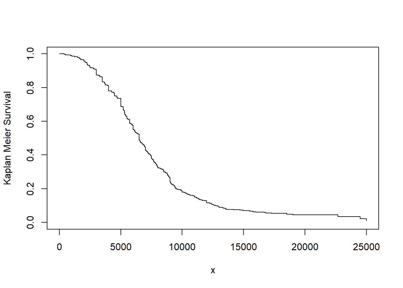
Figure 4.14: Kaplan-Meier Estimate of the Survival Function for Bodily Injury Claims
Show R Code
Right-Censored, Left-Truncated Empirical Distribution Function. In addition to right-censoring, we now extend the framework to allow for left-truncated data. As before, for each observation \(i\), let \(u_i\) be the upper censoring limit (\(=\infty\) if no censoring). Further, let \(d_i\) be the lower truncation limit (0 if no truncation). Thus, the recorded value (if it is greater than \(d_i\)) is \(x_i\) in the case of no censoring and \(u_i\) if there is censoring. Let \(t_{1} <\cdots< t_{k}\) be \(k\) distinct points at which an event of interest occurs, and let \(s_j\) be the number of recorded events \(x_i\)’s at time point \(t_{j}\). The corresponding risk set is \[R_j = \sum_{i=1}^n I(x_i \geq t_{j}) + \sum_{i=1}^n I(u_i \geq t_{j}) - \sum_{i=1}^n I(d_i \geq t_{j}).\]
With this new definition of the risk set, the product-limit estimator of the distribution function is as in equation (4.6).
Greenwood’s Formula. (Greenwood 1926) derived the formula for the estimated variance of the product-limit estimator to be
\[ \widehat{Var}(\hat{F}(x)) = (1-\hat{F}(x))^{2} \sum _{j:t_{j} \leq x} \dfrac{s_j}{R_{j}(R_{j}-s_j)}. \]
As usual, we refer to the square root of the estimated variance as a standard error, a quantity that is routinely used in confidence intervals and for hypothesis testing. To compute this, R‘s survfit method takes a survival data object and creates a new object containing the Kaplan-Meier estimate of the survival function along with confidence intervals. The Kaplan-Meier method (type='kaplan-meier') is used by default to construct an estimate of the survival curve. The resulting discrete survival function has point masses at the observed event times (discharge dates) \(t_j\), where the probability of an event given survival to that duration is estimated as the number of observed events at the duration \(s_j\) divided by the number of subjects exposed or ’at-risk’ just prior to the event duration \(R_j\).
Alternative Estimators. Two alternate types of estimation are also available for the survfit method. The alternative (type='fh2') handles ties, in essence, by assuming that multiple events at the same duration occur in some arbitrary order. Another alternative (type='fleming-harrington') uses the Nelson-AalenA nonparametric estimator of the cumulative hazard function in the presence of incomplete data. (see (Aalen 1978)) estimate of the cumulative hazard function to obtain an estimate of the survival function. The estimated cumulative hazard \(\hat{H}(x)\) starts at zero and is incremented at each observed event duration \(t_j\) by the number of events \(s_j\) divided by the number at risk \(R_j\). With the same notation as above, the Nelson-Äalen estimator of the distribution function is
\[ \begin{aligned} \hat{F}_{NA}(x) &= \left\{ \begin{array}{ll} 0 & x<t_{1} \\ 1- \exp \left(-\sum_{j:t_{j} \leq x}\frac{s_j}{R_j} \right) & x \geq t_{1} \end{array} \right. .\end{aligned} \]
Note that the above expression is a result of the Nelson-Äalen estimator of the cumulative hazard function \[\hat{H}(x)=\sum_{j:t_j\leq x} \frac{s_j}{R_j} \] and the relationship between the survival function and cumulative hazard function, \(\hat{S}_{NA}(x)=e^{-\hat{H}(x)}\).
Example 4.3.7. Actuarial Exam Question.
For observation \(i\) of a survival study:
- \(d_i\) is the left truncation point
- \(x_i\) is the observed value if not right censored
- \(u_i\) is the observed value if right censored
You are given:
\[ {\small \begin{array}{c|cccccccccc} \hline \text{Observation } (i) & 1 & 2 & 3 & 4 & 5 & 6 & 7 & 8 & 9 & 10\\ \hline d_i & 0 & 0 & 0 & 0 & 0 & 0 & 0 & 1.3 & 1.5 & 1.6\\ x_i & 0.9 & - & 1.5 & - & - & 1.7 & - & 2.1 & 2.1 & - \\ u_i & - & 1.2 & - & 1.5 & 1.6 & - & 1.7 & - & - & 2.3 \\ \hline \end{array} } \]
Calculate the Kaplan-Meier product-limit estimate, \(\hat{S}(1.6)\)
Show Example Solution
Example 4.3.8. Actuarial Exam Question. - Continued.
- Using the Nelson-Äalen estimator, calculate the probability that the loss on a policy exceeds 11, \(\hat{S}_{NA}(11)\).
- Calculate Greenwood’s approximation to the variance of the product-limit estimate \(\hat{S}(11)\).
Show Example Solution
Show Quiz Solution
4.4 Bayesian Inference
In this section, you learn how to:
- Describe the Bayesian model as an alternative to the frequentist approach and summarize the five components of this modeling approach.
- Summarize posterior distributions of parameters and use these posterior distributions to predict new outcomes.
- Use conjugate distributions to determine posterior distributions of parameters.
4.4.1 Introduction to Bayesian Inference
Up to this point, our inferential methods have focused on the frequentist setting, in which samples are repeatedly drawn from a population. The vector of parameters \(\boldsymbol \theta\) is fixed yet unknown, whereas the outcomes \(X\) are realizations of random variables.
In contrast, under the BayesianA type of statistical inference in which the model parameters and the data are random variables. framework, we view both the model parameters and the data as random variables. We are uncertain about the parameters \(\boldsymbol \theta\) and use probability tools to reflect this uncertainty.
To get a sense of the Bayesian framework, begin by recalling Bayes’ rule,
\[ \Pr(parameters|data) = \frac{\Pr(data|parameters) \times \Pr(parameters)}{\Pr(data)}, \]
where
- \(\Pr(parameters)\) is the distribution of the parameters, known as the prior distribution.
- \(\Pr(data | parameters)\) is the sampling distribution. In a frequentist context, it is used for making inferences about the parameters and is known as the likelihood.
- \(\Pr(parameters | data)\) is the distribution of the parameters having observed the data, known as the posterior distribution.
- \(\Pr(data)\) is the marginal distribution of the data. It is generally obtained by integrating (or summing) the joint distribution of data and parameters over parameter values.
Why Bayes? There are several advantages of the Bayesian approach. First, we can describe the entire distribution of parameters conditional on the data. This allows us, for example, to provide probability statements regarding the likelihood of parameters. Second, the Bayesian approach provides a unified approach for estimating parameters. Some non-Bayesian methods, such as least squaresA technique for estimating parameters in linear regression. it is a standard approach in regression analysis to the approximate solution of overdetermined systems. in this technique, one determines the parameters that minimize the sum of squared differences between each observation and the corresponding linear combination of explanatory variables., require a separate approach to estimate variance components. In contrast, in Bayesian methods, all parameters can be treated in a similar fashion. This is convenient for explaining results to consumers of the data analysis. Third, this approach allows analysts to blend prior information known from other sources with the data in a coherent manner. This topic is developed in detail in the credibilityAn actuarial method of balancing an individual’s loss experience and the experience in the overall portfolio to improve ratemaking estimates. Chapter 9. Fourth, Bayesian analysis is particularly useful for forecasting future responses.
Gamma - Poisson Special Case. To develop intuition, we consider the gamma-Poisson case that holds a prominent position in actuarial applications. The idea is to consider a set of random variables \(X_1, \ldots, X_n\) where each \(X_i\) could represent the number of claims for the \(i\)th policyholder. Assume that claims of all policyholders follow the same Poisson so that \(X_i\) has a Poisson distribution with parameter \(\lambda\). This is analogous to the likelihood that we first saw in Chapter 2. In a non-Bayesian (or frequentist) context, the parameter \(\lambda\) is viewed as an unknown quantity that is not random (it is said to be “fixed”). In the Bayesian context, the unknown parameter \(\lambda\) is viewed as uncertain and is modeled as a random variable. In this special case, we use the gamma distribution to reflect this uncertainty, the prior distributionThe distribution of the parameters prior to observing data under the bayesian framework..
Think of the following two-stage sampling scheme to motivate our probabilistic set-up.
- In the first stage, the parameter \(\lambda\) is drawn from a gamma distribution.
- In the second stage, for that value of \(\lambda\), there are \(n\) draws from the same (identical) Poisson distribution that are independent, conditional on \(\lambda\).
From this simple set-up, some important conclusions emerge.
- The marginal, or unconditional, distribution of \(X_i\) is no longer Poisson. For this special case, it turns out to be a negative binomial distribution (see the following “Snippet of Theory”).
- The random variables \(X_1, \ldots, X_n\) are not independent. This is because they share the common random variable \(\lambda\).
- As in the frequentist context, the goal is to make statements about likely values of parameters such as \(\lambda\) given the observed data \(X_1, \ldots, X_n\). However, because now both the parameter and the data are random variables, we can use the language of conditional probability to make such statements. As we will see in Section 4.4.4, it turns out that the distribution of \(\lambda\) given the data \(X_1, \ldots, X_n\) is also gamma (with updated parameters), a result that simplifies the task of inferring likely values of the parameter \(\lambda\).
Show A Snippet of Theory
In this section, we use small examples that can be done by hand in order to focus on the foundations. For practical implementation, analysts rely heavily on simulation methods using modern computational methods such as Markov Chain Monte Carlo (MCMC) simulationThe class of numerical methods that use markov chains to generate draws from a posterior distribution.. We will get an exposure to simulation techniques in Chapter 6 but more intensive techniques such as MCMC requires yet more background. See Hartman (2016) for an introduction to computational Bayesian methods from an actuarial perspective.
4.4.2 Bayesian Model
With the intuition developed in the preceding Section 4.4.1, we now restate the Bayesian model with a bit more precision using mathematical notation. For simplicity, we assume both the outcomes and parameters are continuous random variables. In the examples, we sometimes ask the viewer to apply these same principles to discrete versions. Conceptually both the continuous and discrete cases are the same; mechanically, one replaces a pdf by a pmf and an integral by a sum.
To emphasize, under the Bayesian perspective, the model parameters and data are both viewed as random. Our uncertainty about the parameters of the underlying data generating process is reflected in the use of probability tools.
Prior Distribution. Specifically, think about parameters \(\boldsymbol \theta\) as a random vector and let \(\pi(\boldsymbol \theta)\) denote the corresponding mass or density function. This is knowledge that we have before outcomes are observed and is called the prior distribution. Typically, the prior distribution is a regular distribution and so integrates or sums to one, depending on whether \(\boldsymbol \theta\) is continuous or discrete. However, we may be very uncertain (or have no clue) about the distribution of \(\boldsymbol \theta\); the Bayesian machinery allows the following situation
\[ \int \pi(\theta) ~d\theta = \infty, \]
in which case \(\pi(\cdot)\) is called an improper priorA prior distribution in which the sum or integral of the distribution is not finite..
Model Distribution. The distribution of outcomes given an assumed value of \(\boldsymbol \theta\) is known as the model distribution and denoted as \(f(x | \boldsymbol \theta) = f_{X|\boldsymbol \theta} (x|\boldsymbol \theta )\). This is the usual frequentist mass or density function. This is simply the likelihood in the frequentist context and so it is also convenient to use this as a descriptor for the model distribution.
Joint Distribution. The distribution of outcomes and model parameters is a joint distribution of two random quantities. Its joint density function is denoted as \(f(x , \boldsymbol \theta) = f(x|\boldsymbol \theta )\pi(\boldsymbol \theta)\).
Marginal Outcome Distribution. The distribution of outcomes can be expressed as
\[ f(x) = \int f(x | \boldsymbol \theta)\pi(\boldsymbol \theta) ~d \boldsymbol \theta. \]
This is analogous to a frequentist mixture distribution. In the mixture distribution, we combine (or “mix”) different subpopulations. In the Bayesian context, the marginal distribution is a combination of different realizations of parameters (in some literatures, you can think about this as combining different “states of nature”).
Posterior Distribution of Parameters. After outcomes have been observed (hence the terminology “posterior”), one can use Bayes theorem to write the density function as
\[ \pi(\boldsymbol \theta | x) =\frac{f(x , \boldsymbol \theta)}{f(x)} =\frac{f(x|\boldsymbol \theta )\pi(\boldsymbol \theta)}{f(x)} . \]
The idea is to update your knowledge of the distribution of \(\boldsymbol \theta\) (\(\pi(\boldsymbol \theta)\)) with the data \(x\). Making statements about potential values of parameters is an important aspect of statistical inference.
4.4.3 Bayesian Inference
4.4.3.1 Summarizing the Posterior Distribution of Parameters
One way to summarize a distribution is to use a confidence intervalAnother term for interval estimate. unlike a point estimate, it gives a range of reliability for approximating a parameter of interest. type statement. To summarize the posterior distribution of parameters, the interval \([a,b]\) is said to be a \(100(1-\alpha)\%\) credibility intervalA summary of the posterior distribution of parameters under the bayesian framework. for \(\boldsymbol \theta\) if
\[ \Pr (a \le \theta \le b | \mathbf{x}) \ge 1- \alpha. \]
Particularly for insurance applications, this is also known as a credible interval to distinguish it from credibility theory introduced in Chapter 9.
For another approach to summarization, we can look to classical decision analysisBayesian decision theory is the study of an agent’s choices, which is informed by bayesian probability.. In this set-up, the loss function \(l(\hat{\theta}, \theta)\) determines the penalty paid for using the estimate \(\hat{\theta}\) instead of the true \(\theta\). The Bayes estimate is the value that minimizes the expected loss \(\mathrm{E~}[ l(\hat{\theta}, \theta)]\). Some important special cases include:
\[ {\small \begin{array}{cll} \hline \text{Loss function } l(\hat{\theta}, \theta) & \text{Descriptor} & \text{Bayes Estimate} \\ \hline (\hat{\theta}- \theta)^2 & \text{squared error loss} & \mathrm{E}(\theta|X) \\ |\hat{\theta}- \theta| & \text{absolute deviation loss} & \text{median of } \pi(\theta|x) \\ I(\hat{\theta} =\theta) & \text{zero-one loss (for discrete probabilities)} & \text{mode of } \pi(\theta|x) \\ \hline \end{array} } \]
Minimizing expected loss is a rigorous method for providing a single “best guess” about a likely value of a parameter, comparable to a frequentist estimator of the unknown (fixed) parameter.
Example 4.4.1. Actuarial Exam Question. You are given:
- In a portfolio of risks, each policyholder can have at most one claim per year.
- The probability of a claim for a policyholder during a year is \(q\).
- The prior density is \[\pi(q) = q^3/0.07, \ \ \ 0.6 < q < 0.8\]
A randomly selected policyholder has one claim in Year 1 and zero claims in Year 2. For this policyholder, calculate the posterior probability that \(0.7 < q < 0.8\).
Show Example Solution
Example 4.4.2. Actuarial Exam Question. You are given:
- The prior distribution of the parameter \(\Theta\) has probability density function: \[\pi(\theta) = \frac{1}{\theta^2}, \ \ 1 < \theta < \infty\]
- Given \(\Theta = \theta\), claim sizes follow a Pareto distribution with parameters \(\alpha=2\) and \(\theta\).
A claim of 3 is observed. Calculate the posterior probability that \(\Theta\) exceeds 2.
Show Example Solution
4.4.3.2 Bayesian Predictive Distribution
For another type of statistical inference, it is often of interest to “predict” the value of a random outcome that is yet to be observed. Specifically, for new data \(y\), the predictive distributionThe distribution of new data, conditional on a base set of data, under the bayesian framework. is \[ f(y|x) = \int f(y|\theta) \pi(\theta|x) d\theta . \]
It is also sometimes called a “posterior predictive” distribution as the distribution of the new data is conditional on a base set of data.
Using squared error loss for the loss function, the Bayesian prediction of \(Y\) is
\[ \begin{aligned} \mathrm{E}(Y|X) &= \int ~y f(y|X) dy = \int y \left(\int f(y|\theta) \pi(\theta|X) d\theta \right) dy \\ &= \int \left(\int y f(y|\theta) ~dy \right) \pi(\theta|X) ~d\theta \\ &= \int \mathrm{E}(Y|\theta) \pi(\theta|X) ~d\theta . \end{aligned} \] As noted earlier, for some situations the distribution of parameters is discrete, not continuous. Having a discrete set of possible parameters allows us to think of them as alternative “states of nature,” a helpful interpretation.
Example 4.4.3. Actuarial Exam Question. For a particular policy, the conditional probability of the annual number of claims given \(\Theta = \theta\), and the probability distribution of \(\Theta\) are as follows:
\[ {\small \begin{array}{l|ccc} \hline \text{Number of Claims} & 0 & 1 & 2 \\ \text{Probability} & 2\theta & \theta & 1-3\theta \\ \hline \end{array} } \]
\[ {\small \begin{array}{l|cc} \hline \theta & 0.05 & 0.30 \\ \text{Probability} & 0.80 & 0.20 \\ \hline \end{array} } \]
Two claims are observed in Year 1. Calculate the Bayesian prediction of the number of claims in Year 2.
Show Example Solution
Example 4.4.4. Actuarial Exam Question. You are given:
- Losses on a company’s insurance policies follow a Pareto distribution with probability density function: \[ f(x|\theta) = \frac{\theta}{(x+\theta)^2}, \ \ 0 < x < \infty \]
- For half of the company’s policies \(\theta=1\) , while for the other half \(\theta=3\).
For a randomly selected policy, losses in Year 1 were 5. Calculate the posterior probability that losses for this policy in Year 2 will exceed 8.
Show Example Solution
Example 4.4.5. Actuarial Exam Question. You are given:
- The probability that an insured will have at least one loss during any year is \(p\).
- The prior distribution for \(p\) is uniform on \([0, 0.5]\).
- An insured is observed for 8 years and has at least one loss every year.
Calculate the posterior probability that the insured will have at least one loss during Year 9.
Show Example Solution
Example 4.4.6. Actuarial Exam Question. You are given:
- Each risk has at most one claim each year. \[ {\small \begin{array}{ccc} \hline \text{Type of Risk} & \text{Prior Probability} & \text{Annual Claim Probability} \\ \hline \text{I} & 0.7 & 0.1 \\ \text{II} & 0.2 & 0.2 \\ \text{III} & 0.1 & 0.4 \\ \hline \end{array} } \]
One randomly chosen risk has three claims during Years 1-6. Calculate the posterior probability of a claim for this risk in Year 7.
Show Example Solution
4.4.4 Conjugate Distributions
In the Bayesian framework, the key to statistical inference is understanding the posterior distribution of the parameters. As described in Section 4.4.1, modern data analysis using Bayesian methods utilize computationally intensive techniques such as MCMCMarkov Chain Monte Carlo simulation. Another approach for computing posterior distributions are based on conjugate distributions. Although this approach is available only for a limited number of distributions, it has the appeal that it provides closed-form expressions for the distributions, allowing for easy interpretations of results.
To relate the prior and posterior distributions of the parameters, we have the relationship
\[ \begin{array}{ccc} \pi(\boldsymbol \theta | x) & = & \frac{f(x|\boldsymbol \theta )\pi(\boldsymbol \theta)}{f(x)} \\ & \propto & f(x|\boldsymbol \theta ) \pi(\boldsymbol \theta) \\ \text{Posterior} & \text{is proportional to} & \text{likelihood} \times \text{prior} . \end{array} \]
For conjugate distributions, the posterior and the prior belong to the same family of distributions. The following illustration looks at the gamma-Poisson special case, the most well-known in actuarial applications.
Special Case – Gamma-Poisson - Continued. Assume a Poisson(\(\lambda\)) model distribution and that \(\lambda\) follows a gamma(\(\alpha, \theta\)) prior distribution. Then, the posterior distribution of \(\lambda\) given the data follows a gamma distribution with new parameters \(\alpha_{post} = \sum_i x_i + \alpha\) and \(\theta_{post} = 1/(n + 1/\theta)\).
Show Special Case Details
Example 4.4.7. Actuarial Exam Question. You are given:
- The conditional distribution of the number of claims per policyholder is Poisson with mean \(\lambda\).
- The variable \(\lambda\) has a gamma distribution with parameters \(\alpha\) and \(\theta\).
- For policyholders with 1 claim in Year 1, the Bayes prediction for the number of claims in Year 2 is 0.15.
- For policyholders with an average of 2 claims per year in Year 1 and Year 2, the Bayes prediction for the number of claims in Year 3 is 0.20.
Calculate \(\theta\).
Show Example Solution
Closed-form expressions mean that results can be readily interpreted and easily computed; hence, conjugate distributions are useful in actuarial practice. Two other special cases used extensively are:
- The uncertainty of parameters is summarized using a beta distribution and the outcomes have a (conditional on the parameter) binomial distribution.
- The uncertainty about the mean of the normal distribution is summarized using a normal distribution and the outcomes are conditionally normally distributed.
Additional results on conjugate distributions are summarized in the Appendix Section 16.3.
Show Quiz Solution
4.5 Further Resources and Contributors
Exercises
Here are a set of exercises that guide the viewer through some of the theoretical foundations of Loss Data Analytics. Each tutorial is based on one or more questions from the professional actuarial examinations, typically the Society of Actuaries Exam C/STAM.
Contributors
- Edward W. (Jed) Frees and Lisa Gao, University of Wisconsin-Madison, are the principal authors of the initial version of this chapter. Email: jfrees@bus.wisc.edu for chapter comments and suggested improvements.
- Chapter reviewers include: Vytaras Brazauskas, Yvonne Chueh, Eren Dodd, Hirokazu (Iwahiro) Iwasawa, Joseph Kim, Andrew Kwon-Nakamura, Jiandong Ren, and Di (Cindy) Xu.
Bibliography
Aalen, Odd. 1978. “Nonparametric Inference for a Family of Counting Processes.” The Annals of Statistics 6 (4): 701–26.
Box, George E. P. 1980. “Sampling and Bayes’ Inference in Scientific Modelling and Robustness.” Journal of the Royal Statistical Society. Series A (General), 383–430.
Derrig, Richard A, Krzysztof M Ostaszewski, and Grzegorz A Rempala. 2001. “Applications of Resampling Methods in Actuarial Practice.” In Proceedings of the Casualty Actuarial Society, 87:322–64. Casualty Actuarial Society.
Greenwood, Major. 1926. “The Errors of Sampling of the Survivorship Tables.” In Reports on Public Health and Statistical Subjects. Vol. 33. London: Her Majesty’s Stationary Office.
Hartman, Brian. 2016. “Bayesian Computational Methods.” Predictive Modeling Applications in Actuarial Science: Volume 2, Case Studies in Insurance.
James, Gareth, Daniela Witten, Trevor Hastie, and Robert Tibshirani. 2013. An Introduction to Statistical Learning. Vol. 112. Springer.
Kaplan, Edward L., and Paul Meier. 1958. “Nonparametric Estimation from Incomplete Observations.” Journal of the American Statistical Association 53 (282): 457–81.
Picard, Richard R., and Kenneth N. Berk. 1990. “Data Splitting.” The American Statistician 44 (2): 140–47.
Snee, Ronald D. 1977. “Validation of Regression Models: Methods and Examples.” Technometrics 19 (4): 415–28.