Chapter 7 Premium Foundations
Chapter Preview. Setting prices for insurance products, premiums, is an important task for actuaries and other data analysts. This chapter introduces the foundations for pricing non-life products.
7.1 Introduction to Ratemaking
In this section, you learn how to:
- Describe expectations as a baseline method for determining insurance premiums
- Analyze an accounting equation for relating premiums to losses, expenses and profits
- Summarize a strategy for extending pricing to include heterogeneous risks and trends over time
This chapter explains how you can think about determining the appropriate price for an insurance product. As described in Section 1.2, one of the core actuarial functions is ratemakingProcess used by insurers to calculate insurance rates, which drive insurance premiums, where the analyst seeks to determine the right price for a risk.
As this is a core function, let us first take a step back to define terms. A priceA quantity, usually of money, that is exchanged for a good or service is a quantity, usually of money, that is exchanged for a good or service. In insurance, we typically use the word premiumAmount of money an insurer charges to provide the coverage described in the policy for the amount of money charged for insurance protection against contingent events. The amount of protection varies by risk being insured. For example, in homeowners insurance the amount of insurance protection depends on the value of the house. In life insurance, the amount of protection depends on a policyholder’s financial status (e.g. income and wealth) as well as a perceived need for financial security. So, it is common to express insurance prices as a unit of the protection being purchased, for example, a price per thousand dollars of coverage on a home or benefit in the event of death. These prices/premiums are known as ratesA rate is the price, or premium, charged per unit of exposure. a rate is a premium expressed in standardized units. because they are expressed in standardized units,
To determine premiums, it is common in economics to consider the supply and demand of a product. The demand is sensitive to price as well as the existence of competing firms and substitute products. The supply is also sensitive to price as well as the resources required for production. For the individual firm, the price is set to meet some objective such as profit maximization which is met by choosing the output level that balances costs and revenues at the margins.
However, a peculiarity of insurance is that the costs of insurance protection are not known at the sale of the contract. If the insured contingent eventA condition that results in an insurance claim, such as the loss of a house or life, does not occur, then the contract costs are only administrative (to set up the contract) and are relatively minor. If the insured event occurs, then the cost includes not only administrative costs but also payment of the amount insured and expenses to settle claims. So, the cost is random; when the contract is written, by design neither the insurer nor the insured knows the contract costs. Moreover, costs may not be revealed for months or years. For example, a typical time to settlement in medical malpractice is five years.
Because costs are unknown at the time of sale, insurance pricing differs from common economic approaches. This chapter squarely addresses the uncertain nature of costs by introducing traditional actuarial approaches that determine prices as a function of insurance costs. As we will see, this pricing approach is sufficient for some insurance markets such as personal automobile or homeowners where the insurer has a portfolio of many independent risks. However, there are other insurance markets where actuarial prices only provide an input to general market prices. To reinforce this distinction, actuarial cost-based premiums are sometimes known as technical prices. From the perspective of economists, corporate decisions such as pricing are to be evaluated with reference to their impact on the firm’s market value. This objective is more comprehensive than the static notion of profit maximization. That is, you can think of the value of the firm as the capitalized value of all future expected profits. Decisions impacting this value in turn affect all groups having claims on the firm, including stockholders, bondholders, policyowners (in the case of mutual companies), and so forth.
For cost-based prices, it is helpful to think of a premium as revenue source that provides for claim payments, contract expenses, and an operating margin. We formalize this in an accounting equation
\[\begin{equation} \small{ \text{Premium = Loss + Expense + UW Profit} . } \tag{7.1} \end{equation}\]
The Expense term can be split into those that vary by premium (such as sales commissions) and those that do not (such as building costs and employee salaries). The term UW Profit is a residual that stands for underwriting profitProfit an insurer derives from providing coverage, excluding investment income. It may also include include a cost of capital (for example, an annual dividend to company investors). Because fixed expenses and costs of capital are difficult to interpret for individual contracts, we think of the equation (7.1) relationship as holding over the sum of many contracts (a portfolio) and work with it in aggregate. Then, in Section 7.2 we use this approach to help us think about setting premiums, for example by setting profit objectives. Specifically, Sections 7.2.1 and 7.2.2 introduce two prevailing methods used in practice for determining premiums, the pure premiumPure premium is the total severity divided by the number of claims. it does not include insurance company expenses, premium taxes, contingencies, nor an allowance for profits. also called loss costs. some definitions include allocated loss adjustment expenses (alae). and the loss ratioThe sum of losses divided by the premium. methods.
The Loss in equation (7.1) is random and so, as a baseline, we use the expected costs to determine rates. There are several ways to motivate this perspective that we expand upon in Section 7.3. For now, we will suppose that the insurer enters into many contracts with risks that are similar except, by pure chance, in some cases the insured event occurs and in others it does not. The insurer is obligated to pay the total amount of claim payments for all contracts. If risks are similar, then all policyholders are equally likely to contribute to the total loss. So, from this perspective, it makes sense to look at the average claim payment over many insureds. From probability theory, specifically the law of large numbers, we know that the average of iidIndependent and identically distributed risks is close to the expected amount, so we use the expectation as a baseline pricing principle.
Nonetheless, by using expected losses, we essentially assume that the uncertainty is non-existent. If the insurer sells enough independent policies, this may be a reasonable approximation. However, there will be other cases, such as a single contract issued to a large corporation to insure all of its buildings against fire damage, where the use of only an expectation for pricing is not sufficient. So, Section 7.3 also summarizes alternative premium principles that incorporate uncertainty into our pricing. Note that an emphasis of this text is estimation of the entire distribution of losses so the analyst is not restricted to working only with expectations.
The aggregate methods derived from equation (7.1) focus on collections of homogeneous risksRisks that have the same distribution, that is, the distributions are identical. that are similar except for the occurrence of random losses. In statistical language that we have introduced, this is a discussion about risks that have identical distributions. Naturally, when examining risks that insurers work with, there are many variations in the risks being insured including the features of the contracts and the people being insured. Section 7.4 extends pricing considerations to heterogeneousHeterogeneous risks have different distributions. often, we can attribute differences to varying exposures or risk factors. collections of risks.
Section 7.5 introduces development and trending. When developing rates, we want to use the most recent loss experience because the goal is to develop rates that are forward looking. However, at contract initiation, recent loss experience is often not known; it may be several years until it is fully realized. So, this section introduces concepts needed for incorporating recent loss experience into our premium development. Development and trending of experience is related to but also differs from the idea of experience ratingA type of rating plan that uses the insured’s historical loss experience as part of the premium determination that suggests that experience reveals hidden information about the insured and so should be incorporated in our forward thinking viewpoint. Chapter 9 discusses this idea in more detail.
The final section of this chapter introduces methods for selecting a premium. This is done by comparing a premium rating method to losses from a held-out portfolio and selecting the method that produces the best match with the held-out data. For a typical insurance portfolio, most policies produce zero losses, that is, do not have a claim. Because the distribution of held-out losses is a combination of (a large number of) zeros and continuous amounts, special techniques are useful. Section 7.6 introduces concepts of concentration curves and corresponding Gini statistics to help in this selection.
The chapter also includes a technical supplement on government regulation of insurance ratesAmount of money needed to cover losses, expenses, and profit per one unit of exposure to keep our work grounded in applications.
7.2 Aggregate Ratemaking Methods
In this section, you learn how to:
- Define a pure premium as a loss cost as well as in terms of frequency and severity
- Calculate an indicated rate using pure premiums, expenses, and profit loadings
- Define a loss ratio
- Calculate an indicated rate change using loss ratios
- Compare the pure premium and loss ratio methods for determining premiums
It is common to consider an aggregate portfolio of insurance experience. Consistent with earlier notation, consider a collection of \(n\) contracts with losses \(X_1, \ldots, X_n\). In this section, we assume that contracts have the same loss distribution, that is they form a homogeneous portfolio, and so are iidIndependent and identically distributed. For motivation, you can think about personal insurance such as auto or homeowners where insurers write many contracts on risks that appear very similar. Further, the assumption of identical distributions is not as limiting as you might think. In Section 7.4.1 we will introduce the idea of an exposureA type of rating variable that is so important that premiums and losses are often quoted on a “per exposure” basis. that is, premiums and losses are commonly standardized by exposure variables. variable that allows us to rescale experience to make it comparable. For example, by rescaling losses we will be able to treat homeowner losses from a house with 80,000 insurable value and a house with a 320,000 insurable value as coming from the same distribution. For now, we simply assume that \(X_1, \ldots, X_n\) are iid.
7.2.1 Pure Premium Method
If the number of policies in a collection, \(n\), is large, then the average provides a good approximation of the expected loss \[ \small{ \mathrm{E}(X) \approx \frac{\sum_{i=1}^n X_i}{n} = \frac{\text{Loss}}{\text{Exposure}} = \text{Pure Premium}. } \] With this as motivation, we define the pure premiumPure premium is the total severity divided by the number of claims. it does not include insurance company expenses, premium taxes, contingencies, nor an allowance for profits. also called loss costs. some definitions include allocated loss adjustment expenses (alae). to be the sum of losses divided by the exposure; it is also known as a loss costThe sum of losses divided by an exposure; it is also known as the pure premium.. In the case of homogeneous risksRisks that have the same distribution, that is, the distributions are identical., all policies are treated the same and we can use the number of policies \(n\) for the exposure. In Section 7.4.1 we extend the concept of exposure when policies are not the same.
We can multiply and divide by the number of claims, claim count, to get
\[
\small{
\text{Pure Premium} = \frac{\text{claim count}}{\text{Exposure}} \times \frac{\text{Loss}}{\text{claim count}} = \text{frequency} \times \text{severity} .
}
\]
So, when premiums are determined using the pure premium method, we either take the average loss (loss cost) or use the frequency-severity approach.
To get a bit closer to applications in practice, we now return to equation (7.1) that includes expenses. Equation (7.1) also refers to UW Profit for underwriting profit. When rescaled by premiums, this is known as the profit loadingA factor or percentage applied to the premium calculation to account for insurer profit in a policy. Because claims are uncertain, the insurer must hold capital to ensure that all claims are paid. Holding this extra capital is a cost of doing business, investors in the company need to be compensated for this, thus the extra loading.
We now decompose Expenses into those that vary by premium, Variable, and those that do not, Fixed so that Expenses = Variable + Fixed. Thinking of variable expenses and profit as a fraction of premiums, we define
\[ \small{ V = \frac{\text{Variable}}{\text{Premium}} ~~~ \text{and}~~~ Q = \frac{\text{UW Profit}}{\text{Premium}} ~. } \]
With these definitions and equation (7.1), we may write \[ \small{ \begin{matrix} \begin{array}{ll} \text{Premium} &= \text{Losses + Fixed} + \text{Premium} \times \frac{\text{Variable + UW Profit}}{\text{Premium}} \\ & = \text{Losses + Fixed} + \text{Premium} \times (V+Q) . \end{array} \end{matrix} } \] Solving for premiums yields
\[\begin{equation} \small{ \text{Premium} = \frac{\text{Losses + Fixed}}{1-V-Q} . } \tag{7.2} \end{equation}\]
Dividing by exposure, the rate can be calculated as
\[ \begin{matrix} \begin{array}{ll} \text{Rate} &= \frac{\text{Premium}}{\text{Exposure}} = \frac{\text{Losses/Exposure + Fixed/Exposure}}{1-V-Q} \\ &= \frac{\text{Pure Premium + Fixed/Exposure}}{1-V-Q} ~. \end{array} \end{matrix} \]
In words, this is
\[ \small{ \text{Rate} =\frac{\text{pure premium + fixed expense per exposure}}{\text{1 - variable expense factor - profit and contingencies factor}} . } \]
Example. CAS Exam 5, 2004, Number 13. Determine the indicated rateIn a rate filing, the amount that the loss experience suggests that the insurer should charge to cover costs. per exposure unit, given the following information:
- Frequency per exposure unit = 0.25
- Severity = $100
- Fixed expense per exposure unit = $10
- Variable expense factor = 20%
- Profit and contingencies factor = 5%
Show Example Solution
From the example, note that the rates produced by the pure premium method are commonly known as indicated rates.
From our development, note also that the profit is associated with the underwriting aspect of the contract and not investments. Premiums are typically paid at the beginning of a contract and insurers receive investment income from holding this money. However, due in part to the short-term nature of the contracts, investment income is typically ignored in pricing. This builds a bit of conservatism into the process that insurers welcome. It is probably most relevant in the very long “tail” lines such as workers’ compensation and medical malpractice. In these lines, it can sometimes take 20 years or even longer to settle claims. But, these are also the most volatile lines with some claim amounts being large relative to the rest of the distribution. The mitigating factor is that these large claim amounts tend to be far in the future and so are less extreme when viewed in a discounted sense.
7.2.2 Loss Ratio Method
The loss ratioThe sum of losses divided by the premium. is the ratio of the sum of losses to the premium
\[ \small{ \text{Loss Ratio} = \frac{\text{Loss}}{\text{Premium}} . } \]
When determining premiums, it is a bit counter-intuitive to emphasize this ratio because the premium component is built into the denominator. As we will see, the loss ratio method develops rate changes rather than rates; we can use rate changes to update past experience to get a current rate. To do this, rate changes consist of the ratio of the experience loss ratio to the target loss ratio. This adjustment factor is then applied to current rates to get new indicated rates.
To see how this works in a simple context, let us return to equation (7.1) but now ignore expenses to get \(\small{\text{Premium = Losses + UW Profit}}\). Dividing by premiums yields
\[ \small{ \frac{\text{UW Profit}}{\text{Premium}} = 1 - LR = 1 - \frac{\text{Loss}}{\text{Premium}} . } \] Suppose that we have in mind a new “target” profit loading, say \(Q_{target}\). Assuming that losses, exposure, and other things about the contract stay the same, then to achieve the new target profit loading we adjust the premium. Use the ICF for the indicated change factorA factor calculated from the loss ratio method that calculates how the rates should change, with factors > 1 indicating an increase and vice versa that is defined through the expression
\[ \small{ \frac{\text{New UW Profit}}{\text{Premium}} = Q_{target} = 1 - \frac{\text{Loss}}{ICF \times \text{Premium}}. } \] Solving for ICF, we get
\[ \small{ ICF = \frac{\text{Loss}}{\text{Premium} \times (1-Q_{target})} = \frac{LR}{1-Q_{target}}. } \]
So, for example, if we have a current loss ratio = 85% and a target profit loading \(\small{Q_{target}=0.20}\), then \(\small{ICF = 0.85/0.80 = 1.0625}\), meaning that we increase premiums by 6.25%.
Now let’s see how this works with expenses in equation (7.1). We can use the same development as in Section 7.2.1 and so start with equation (7.2), solve for the profit loading to get
\[
\small{
Q = 1 - \frac{\text{Loss+Fixed}}{\text{Premium}} - V .
}
\]
We interpret the quantity Fixed /Premium + V as the “operating expense ratio.” Now, fix the profit percentage Q at a target and adjust premiums through the “indicated change factor” \(ICF\)
\[
\small{
Q_{target} = 1
-\frac{\text{Loss + Fixed}}{\text{Premium}\times ICF} - V .
}
\]
Solving for \(ICF\) yields
\[\begin{equation} {\small \begin{array}{ll} ICF &= \frac{\text{Loss + Fixed}}{\text{Premium} \times (1 - V - Q_{target})} \\ &= \frac{\text{Loss Ratio + Fixed Expense Ratio}}{1 - V - Q_{target}} . \end{array} \tag{7.3} } \end{equation}\]
Example. Loss Ratio Indicated Change Factor. Assume the following information:
- Projected ultimate loss and LAE ratio = 65%
- Projected fixed expense ratio = 6.5%
- Variable expense = 25%
- Target UW profit = 10%
With these assumptions, with equation (7.3), the indicated change factor can be calculated as \[ \small{ ICF = \frac{\text{(Losses + Fixed)}/\text{Premium}}{ 1 - V - Q_{target}} = \frac{0.65 + 0.065}{1- 0.25 - 0.10} = 1.10 . } \]
This means that overall average rate level should be increased by 10%.
We later provide a comparison of the pure premium and loss ratio methods in Section 7.5.3. As inputs, that section will require discussions of trended exposures and on-level premiums defined in Section 7.5.
7.3 Pricing Principles
In this section, you learn how to:
- Describe common actuarial pricing principles
- Describe properties of pricing principles
- Choose a pricing principle based on a desired property
Approaches to pricing vary by the type of contract. For example, personal automobile is a widely available product throughout the world and is known as part of the retail general insurance market in the United Kingdom. Here, one can expect to do pricing based on a large pool of independent contracts, a situation in which expectations of losses provide an excellent starting point. In contrast, an actuary may wish to price an insurance contract issued to a large employer that covers complex health benefits for thousands of employees. In this example, knowledge of the entire distribution of potential losses, not just the expected value, is critical for starting the pricing negotiations. To cover a range of potential applications, this section describes general premium principles and their properties that one can use to decide whether or not a specific principle is applicable in a given situation.
7.4 Heterogeneous Risks
In this section, you learn how to:
- Describe insurance exposures in terms of scale distributions
- Explain an exposure in terms of common types of insurance such as auto and homeowners insurance
- Describe how rating factors can be used to account for the heterogeneity among risks in a collection
- Measure the impact of a rating factor through relativities
As noted in Section 7.1, there are many variations in the risks being insured, the features of the contracts, and the people being insured. As an example, you might have a twin brother or sister who works in the same town and earns a roughly similar amount of money. Still, when it comes to selecting choices in rental insurance to insure contents of your apartment, you can imagine differences in the amount of contents to be insured, choices of deductibles for the amount of risk retained, and perhaps different levels of uncertainty given the relative safety of your neighborhoods. People and risks that they insure are different.
When thinking about a collection of different (heterogeneousHeterogeneous risks have different distributions. often, we can attribute differences to varying exposures or risk factors.) risks, one option is to price all risks the same. This is common in government sponsored programs for flood or health insurance. However, it is also common to have different prices where the differences are commensurate with the risk being insured.
7.4.1 Exposure to Risk
One way to make heterogeneous risks comparable is through the concept of an exposureA type of rating variable that is so important that premiums and losses are often quoted on a “per exposure” basis. that is, premiums and losses are commonly standardized by exposure variables.. To explain exposures, let us use scale distributions that we learned about in Chapter 3. To recall a scale distributionSuppose that y = c x, where x comes from a parametric distribution family and c is a positive constant. the distribution is said to be a scale distribution if (i) the distributions of y and x come from the same family and (ii) only a single parameter differs and that by a factor of c., suppose that \(X\) has a parametric distributionModel assumption that the sample data comes from a population that can be modeled by a probability distribution with a fixed set of parameters and define a rescaled version \(R = X/E\), \(E > 0\). If \(R\) is in the same parametric family as \(X\), then the distribution is said to be a scale distribution. As we have seen, the gamma, exponential, and Pareto distributions are examples of scale distributions.
Intuitively, the idea behind exposures is to make risks more comparable to one another. For example, it may be that risks \(X_1, \ldots, X_n\) come from different distributions and yet, with the choice of the right exposures, the rates \(R_1, \ldots, R_n\) come from the same distribution. Here, we interpret the rate \(R_i = X_i/E_i\) to be the loss divided by exposure.
Table 7.3 provides a few examples. We remark that this table refers to “earned” car and house years, concepts that will be explained in Section 7.5.
Table 7.3. Commonly used Exposures in Different Types of Insurance
\[ \small{ \begin{matrix} \begin{array}{ll} \text{Type of Insurance} & \text{Exposure Basis} \\\hline \text{Personal Automobile} & \text{Earned Car Year, Amount of Insurance Coverage} \\ \text{Homeowners} & \text{Earned House Year, Amount of Insurance Coverage}\\ \text{Workers Compensation} & \text{Payroll}\\ \text{Commercial General Liability} & \text{Sales Revenue, Payroll, Square Footage, Number of Units}\\ \text{Commercial Business Property} & \text{Amount of Insurance Coverage}\\ \text{Physician's Professional Liability} & \text{Number of Physician Years}\\ \text{Professional Liability} & \text{Number of Professionals (e.g., Lawyers or Accountants)}\\ \text{Personal Articles Floater} & \text{Value of Item} \\ \hline \end{array} \end{matrix} } \]
An exposure is a type of rating factorA rating factor, or rating variable, is a characteristic of the policyholder or risk being insured by which rates vary., a concept that we define explicitly in the next Section 7.4.2. It is typically the most important rating factor, so important that both premiums and losses are quoted on a “per exposure” basis.
For frequency and severity modeling, it is customary to think about the frequency aspect as proportional to exposure and the severity aspect in terms of loss per claim (not dependent upon exposure). However, this does not cover the entire story. For many lines of business, it is convenient for exposures to be proportional to inflation. Inflation is typically viewed as unrelated to frequency but proportional to severity.
Criteria for Choosing an Exposure
An exposure base should meet the following criteria. It should:
- be an accurate measure of the quantitative exposure to loss
- be easy for the insurer to determine (at the time the policy is initiated) and not subject to manipulation by the insured,
- be easy to understand by the insured and to calculate by the insurer,
- consider any preexisting exposure base established within the industry, and
- for some lines of business, be proportional to inflation. In this way, rates are not sensitive to the changing value of money over time as these changes are captured in exposure base.
To illustrate, consider personal automobile coverage. Instead of the exposure basis “earned car year,” a more accurate measure of the quantitative exposure to loss might be number of miles driven. Historically, this measure had been difficult to determine at the time the policy is issued and subject to potential manipulation by the insured and so it is still not typically used. Modern telematic devices that allow for accurate mileage recording is changing the use of this variable in some marketplaces.
As another example, the exposure measure in commercial business propertyLine of business that insures against damage to their buildings and contents due to a covered cause of loss, e.g. fire insurance, is typically the amount of insurance coverage. As property values grow with inflation, so will the amount of insurance coverage. Thus, rates quoted on a per amount of insurance coverage are less sensitive to inflation than otherwise.
7.4.2 Rating Factors
A rating factor, or rating variableA rating factor, or rating variable, is a characteristic of the policyholder or risk being insured by which rates vary., is simply a characteristic of the policyholder or risk being insured by which rates vary. For example, when you purchase auto insurance, it is likely that the insurer has rates that differ by age, gender, type of car, where the car is garaged, accident history, and so forth. These variables are known as rating factors. Although some variables may be continuous, such as age, most are categorical - factorA variable that varies by groups or categories. is a label that is used for categorical variables. In fact, even with continuous variablesType of variable that can take on any real value such as age, it is common to categorize them by creating groups such as “young,” “intermediate,” and “old” for rating purposes.
Table 7.4 provides just a few examples. In many jurisdictions, the personal insurance market (e.g., auto and homeowners) is very competitive - using 10 or 20 variables for rating purposes is not uncommon.
Table 7.4. Commonly used Rating Factors in Different Types of Insurance
\[ \small{ \begin{matrix} \begin{array}{l|l}\hline \text{Type of Insurance} & \text{Rating Factors}\\\hline\hline \text{Personal Automobile} & \text{Driver Age and Gender, Model Year, Accident History}\\ \text{Homeowners} & \text{Amount of Insurance, Age of Home, Construction Type}\\ \text{Workers Compensation} & \text{Occupation Class Code}\\ \text{Commercial General Liability} & \text{Classification, Territory, Limit of Liability}\\ \text{Medical Malpractice} & \text{Specialty, Territory, Limit of Liability}\\ \text{Commercial Automobile} & \text{Driver Class, Territory, Limit of Liability}\\ \hline \end{array} \end{matrix} } \]
Example. Losses and Premium by Amount of Insurance and Territory. To illustrate, Table 7.5 presents a small fictitious data set from Werner and Modlin (2016). The data consists of loss and loss adjustment expenses (LossLAE), decomposed by three levels of amount of insurance (AOI), and three territories (Terr). For each combination of AOI and Terr, we also have available the number of policies issued, given as the Exposure.
Table 7.5. Losses and Premium by Amount of Insurance and Territory
\[ \small{ \begin{matrix} \begin{array}{cc|rrr} \hline AOI & Terr & Exposure & LossLAE & Premium \\\hline \text{Low} & 1 & 7 & 210.93 & 335.99 \\ \text{Medium} & 1 & 108 & 4,458.05 & 6,479.87 \\ \text{High} & 1 & 179 & 10,565.98 & 14,498.71 \\\hline \text{Low} & 2 & 130 & 6,206.12 & 10,399.79 \\ \text{Medium} & 2 & 126 & 8,239.95 & 12,599.75 \\ \text{High} & 2 & 129 & 12,063.68 & 17,414.65 \\\hline \text{Low} & 3 & 143 & 8,441.25 & 14,871.70 \\ \text{Medium} & 3 & 126 & 10,188.70 & 16,379.68 \\ \text{High} & 3 & 40 & 4,625.34 & 7,019.86 \\ \hline \text{Total} & & 988 & 65,000.00 & 99,664.01 \\\hline \hline \end{array} \end{matrix} } \]
In this case, the rating factors AOI and Terr produce nine cells. Note that one might combine the cell “territory one with a low amount of insurance”" with another cell because there are only 7 policies in that cell. Doing so is perfectly acceptable - considerations of this sort is one of the main jobs of the analyst. An outline on selecting variables is in Chapter 8, including Technical Supplement TS 8.B. Alternatively, you can also think about reinforcing information about the cell (Terr 1, Low AOI) by “borrowing” information from neighboring cells (e.g., other territories with the same AOI, or other amounts of AOI within Terr 1). This is the subject of credibilityWeight assigned to observed data vs. that assigned to an external or broader-based set of data that is introduced in Chapter 9.
To understand the impact of rating factors, it is common to use relativities. A relativityThe difference of the expected risk between a specific level of a rating factor and an accepted baseline value. this difference may be arithmetic or proportional. compares the expected risk at a specific level of a rating factor to an accepted baseline value. In this book, we work with relativities defined through ratios; it is also possible to define relativities through arithmetic differences. Thus, our relativity is defined as
\[ \text{Relativity}_j = \frac{\text{(Loss/Exposure)}_j}{\text{(Loss/Exposure)}_{Base}} . \]
Example. Losses and Premium by Amount of Insurance and Territory - Continued. Traditional classification methods consider only one classification variable at a time - they are univariate. Thus, if we wanted relativities for losses and expenses (LossLAE) by amount of insurance, we might sum over territories to get the information displayed in Table 7.6.
Table 7.6. Losses and Relativities by Amount of Insurance
\[ \small{ \begin{matrix} \begin{array}{c|rrrr} \hline AOI & Exposure & LossLAE & Loss/Exp &Relativity \\\hline \text{Low} & 280 & 14858.3 & 53.065 &0.835 \\ \text{Medium} & 360 & 22886.7 & 63.574 &1.000 \\ \text{High} & 348 & 27255.0 & 78.319 & 1.232 \\\hline \text{Total} & 988 & 65,000.0 & \\\hline \hline \end{array} \end{matrix} } \]
Thus, losses and expenses per unit of exposure are 23.2% higher for risks with a high amount of insurance compared to those with a medium amount. These relativities do not control for territory.
The introduction of rating factors allows the analyst to create cells that define small collections of risks – the goal is to choose the right combination of rating factors so that all risks within a cell may be treated the same. In statistical terminology, we want all risks within a cell to have the same distribution (subject to rescaling by an exposure variable). This is the foundation of insurance pricing. All risks within a cell have the same price per exposure yet risks from different cells may have different prices.
Said another way, insurers are allowed to charge different rates for different risks; discriminationProcess of determining premiums on the basis of likelihood of loss. insurance laws prohibit “unfair discrimination”. of risks is legal and routinely done. Nonetheless, the basis of discrimination, the choice of risk factors, is the subject of extensive debate. The actuarial community, insurance management, regulators, and consumer advocates are all active participants in this debate. Technical Supplement TS 7.A describes these issues from a regulatory perspective.
In addition to statistical criteria for assessing the significance of a rating factor, analysts much pay attention to business concerns of the company (e.g., is it expensive to implement a rating factor?), social criteria (is a variable under the control of a policyholder?), legal criteria (are there regulations that prohibit the use of a rating factor such as gender?), and other societal issues. These questions are largely beyond the scope of this text. Nonetheless, because they are so fundamental to pricing of insurance, a brief overview is given in Chapter 8, including Technical Supplement TS 8.B.
7.5 Development and Trending
In this section, you learn how to:
- Define and calculate different types of exposure and premium summary measures that appear in financial reports
- Describe the development of a claim over several payments and link that to various unpaid claim measures, including incurred but not reported (IBNR) as well as case reserves
- Compare and contrast relative strengths and weaknesses of the pure premium and loss ratio methods for ratemaking
As we have seen in Section 7.2, insurers consider aggregate information for ratemaking such as exposures to risk, premiums, expenses, claims, and payments. This aggregate information is also useful for managing an insurers’ activities; financial reports are commonly created at least annually and oftentimes quarterly. At any given financial reporting date, information about recent policies and claims will be ongoing and necessarily incomplete; this section introduces concepts for projecting risk information so that it is useful for ratemaking purposes. Information about the risks, such as exposures, premium, claim counts, losses, and rating factors, is typically organized into three databases:
- policy database - contains information about the risk being insured, the policyholder, and the contract provisions
- claims database - contains information about each claim; these are linked to the policy database.
- payment database - contains information on each claims transaction, typically payments but may also changes to case reserves. These are linked to the claims database.
With these detailed databases, it is straightforward (in principle) to sum up policy level detail to aggregate information needed for financial reports. This section describes various summary measures commonly used.
7.5.1 Exposures and Premiums
A financial reporting period is a length of time that is fixed in the calendar; we use January 1 to December 31 for the examples in this book although other reporting periods are also common. The reporting period is fixed but policies may begin at any time during the year. Even if all policies have a common contract length of (say) one year, because of the differing starting time, they can end at any time during the financial reporting. Figure 7.1 presents four illustrative policies. There need to be some standards as to what types of measures are most useful for summarizing experience in a given reporting period due to these differing start and end times.
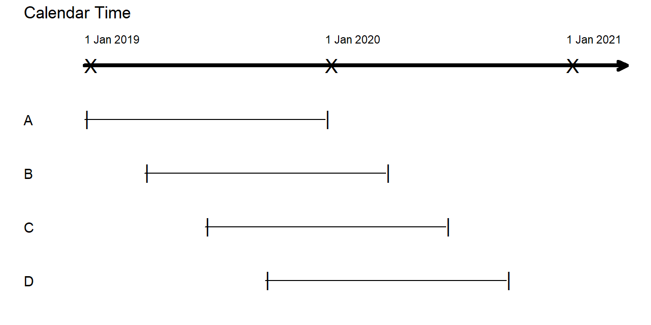
Figure 7.1: Timeline of Exposures for Four 12-Month Policies
Some commonly used exposure measures are:
- written exposuresExposure is based off policies written/issued, the amount of exposures on policies issued (underwritten or written) during the period in question,
- earned exposuresExposure is based off amount exposed to loss for which coverage has been provided, the exposure units actually exposed to loss during the period, that is, where coverage has already been provided
- unearned exposuresExposure amount for which coverage has not yet been provided, represent the portion of the written exposures for which coverage has not yet been provided as of that point in time, and
- in force exposuresExposure amount subject to loss at a particular point in time, exposure units exposed to loss at a given point in time.
Table 7.7 gives detailed illustrative calculations for the four illustrative policies.
Table 7.7. Exposures for Four 12-Month Policies
\[ \small{ \begin{matrix} \begin{array}{cl|cc|cc|cc|c} \hline & & & & & & &&\text{In-Force} \\ &\text{Effective} & \text{Written}& \text{Exposure} & \text{Earned} &\text{Exposure}& \text{Unearned} &\text{Exposure}& \text{Exposure} \\ {Policy} &\text{Date} & 1/1/2019 & 1/1/2020 & 1/1/2019 & 1/1/2020 & 1/1/2019 & 1/1/2020 & 1/1/2020 \\ \hline \text{A}&\text{1 Jan 2019} & 1.00 & 0.00 & 1.00 & 0.00& 0.00 & 0.00 & 0.00 \\ \text{B}&\text{1 April 2019} & 1.00 & 0.00 & 0.75 & 0.25 & 0.25 & 0.00& 1.00 \\ \text{C}&\text{1 July 2019} & 1.00 & 0.00 & 0.50 & 0.50 & 0.50 & 0.00& 1.00 \\ \text{D}&\text{1 Oct 2019} & 1.00 & 0.00 & 0.25 & 0.75 & 0.75 & 0.00& 1.00 \\ \hline & Total & 4.00 & 0.00 & 2.50 & 1.50 & 1.50 & 0.00 & 3.00 \\ \hline \hline \end{array} \end{matrix} } \]
This summarization is sometimes known as the calendar year methodExperience for rating is aggregated based on calendar year, as opposed to other methods such as when a policy term began of aggregation to serve as a contrast to the policy yearThis is the period between a policy’s anniversary dates. method. In the policy year method, all premiums and losses for policies written in the policy year are aggregated regardless of when earned. For example, for all four policies A, B, C, and D, they have written and earned exposures of 1.00 for the policy year 2019 (starting on 1/1 or 1 Jan). This is despite the fact that they do not start at the beginning of the year. This method is useful for ratemaking methods based on individual contracts and we do not pursue this further here.
In the same way as exposures, one can summarize premiums. Premiums, like exposures, can be either written, earned, unearned, or in force. Consider the following example.
Example 7.5.1. CAS Exam 5, 2003, Number 10. A 12-month policy is written on March 1, 2002 for a premium of $900. As of December 31, 2002, which of the following is true?
\[ \small{ \begin{matrix} \begin{array}{l|ccc} \hline & \text{Calendar Year} & \text{Calendar Year} \\ & \text{2002 Written} & \text{2002 Earned} & \text{Inforce} \\ & \text{Premium} & \text{Premium} & \text{Premium} \\\hline A. & 900 & 900 & 900 \\ B. & 750 & 750 & 900 \\ C. & 900 & 750 & 750 \\ D. & 750 & 750 & 750 \\ E. & 900 & 750 & 900 \\\hline \end{array} \end{matrix} } \]
Show Example Solution
7.5.2 Losses, Claims, and Payments
Broadly speaking, the terms lossThe amount of damages sustained by an individual or corporation, typically as the result of an insurable event. and claimThe amount paid to an individual or corporation for the recovery, under a policy of insurance, for loss that comes within that policy. refer to the amount of compensation paid or potentially payable to the claimant under the terms of the insurance policy. Definitions can vary:
- Sometimes, the term claim is used interchangeably with the term loss.
- In some insurance and actuarial sources, the term loss is used for the amount of damage sustained in an insured event. The claim is the amount paid by the insurer with differences typically due to deductibles, upper policy limits, and the like.
- In economics, a claim is a demand for payment by an insured or by an injured third-party under the terms and conditions of insurance contract and the loss is the amount paid by the insurer.
This text will follow the second bullet. However, when reading other sources, you will need to take care when thinking about definitions for the terms loss and claim.
To establish additional terminology, it is helpful to follow the timeline of a claim as it develops. In Figure 7.2, the claim occurs at time \(t_1\) and the insuring company is notified at time \(t_3\). There can be a long gap between occurrence and notification such that the end of a company financial reporting period, known as a valuation dateA valuation date is the date at which a company summarizes its financial position, typically quarterly or annually., occurs (\(t_2\)) before the loss is reported. In this case, the claim is said to be incurred but not reportedA claim is said to be incurred but not reported if the insured event occurs prior to a valuation date (and hence the insurer is liable for payment) but the event has not been reported to the insurer. at this valuation date.
After claim notification, there may one or more loss payments. Not all of the payments may be made by the next valuation date (\(t_4\)). As the claim develops, eventually the company deems its financial obligations on the claim to be resolved and declares the claim closedA claim is said to be closed when the company deems its financial obligations on the claim to be resolved.. However, it is possible that new facts arise and the claim must be re-opened, giving rise to additional loss payments prior to being closed again.
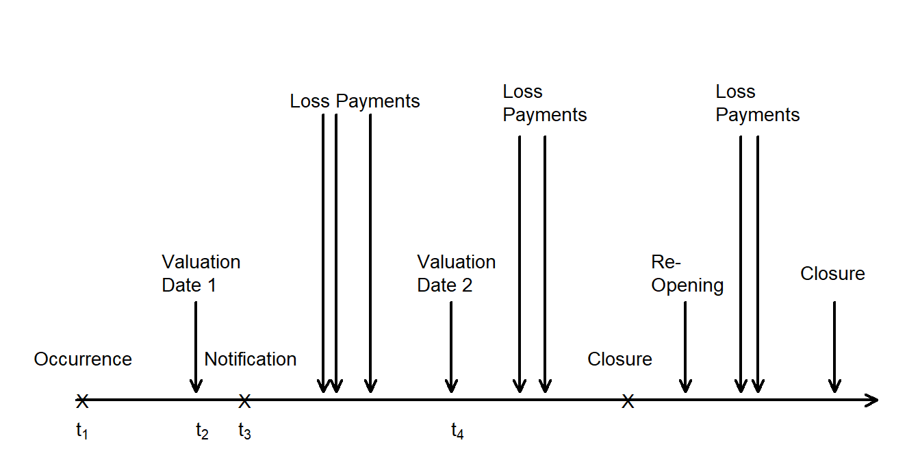
Figure 7.2: Timeline of Claim Development
- Accident dateDate of loss occurrence that gives rise to a claim - the date of the occurrence which gave rise to the claim. This is also known as the date of loss or the occurrence date.
- Report dateDate when insurer is notified of the claim - the date the insurer receives notice of the claim. Claims not currently known by the insurer are referred to as unreported claims or incurred but not reported (IBNR) claims.
Until the claim is settled, the reported claim is considered an open claimA claim that has been reported but not yet closed. Once the claim is settled, it is categorized as a closed claim. In some instances, further activity may occur after the claim is closed, and the claim may be re-opened.
Recall that a claim is the amount paid or payable to claimants under the terms of insurance policies. Further, we have
- Paid losses are those losses for a particular period that have actually been paid to claimants.
- Where there is an expectation that payment will be made in the future, a claim will have an associated case reserve representing the estimated amount of that payment.
- Reported Losses, also known as case incurred, is Paid Losses + Case Reserves
The ultimate loss is the amount of money required to close and settle all claims for a defined group of policies.
7.5.3 Comparing Pure Premium and Loss Ratio Methods
Now that we have learned how exposures, premiums, and claims develop over time, we can consider how they can be used for ratemaking. We have seen that insurers offer many different types of policies that cover different policyholders and amounts of risks. This aggregation is sometimes loosely referred to as the mix of businessDifferent types of policies in an insurer’s portfolio. Importantly, the mix changes over time as policyholders come and go, amounts of risks change, and so forth. The exposures, premiums, and types of risks from a prior financial reporting may not be representative of the period for which the rates are being developed. The process of extrapolating exposures, premiums, and risk types is known as trending. For example, an on-level earned premiumEarned premium of historical policies using the current rate structure is that earned premium that would have resulted for the experience period had the current rates been in effect for the entire period; this is also known as an earned premium at current rates. Most trending methods used in practice are mathematically straight-forward although they can become complicated given contractual and administrative complexities. We refer the reader to standard references that describe approaches in detail such as Werner and Modlin (2016) and Friedland (2013).
Loss Ratio Method
The expression for the loss ratio method indicated change factor in equation (7.3) assumes a certain amount of consistency in the portfolio experience over time. For another approach, we can define the experience loss ratioRatio of experience loss to on-level earned premium in the experience period to be:
\[ \small{ LR_{experience} = \frac{\text{experience losses}}{\text{experience period earned exposure}\times \text{current rate}} . } \]
Here, we think of the experience period earned exposure \(\times\) current rate as the experience premium.
Using equation (7.2), we can write a loss ratio as
\[ \small{ LR = \frac{\text{Losses}}{\text{Premium}}=\frac{1-V-Q}{\text{(Losses + Fixed)}/\text{Losses}}=\frac{1-V-Q}{1+G} ~, } \] where \(G = \text{Fixed} / \text{Losses}\), the ratio of fixed expenses to losses. With this expression, we define the target loss ratio
\[ \small{ LR_{target} = \frac{1-V-Q}{1+G} = \frac{1-\text{premium related expense factor - profit and contingencies factor}} {1+\text{ratio of non-premium related expenses to losses}} . } \]
With these, the indicated change factor is
\[\begin{equation} \small{ ICF =\frac{LR_{experience}}{LR_{target}}. } \tag{7.4} \end{equation}\]
Comparing equation (7.3) to (7.4), we see that the latter offers more flexibility to explicitly incorporate trended experience. As the loss ratio method is based on rate changes, this flexibility is certainly warranted.
Comparison of Methods
Assuming that exposures, premiums, and claims have been trended to be representative of a period that rates are being developed for, we are now in a position to compare the pure premium and loss ratio methods for ratemaking. We start with the observation that for the same data inputs, these two approaches produce the same results. That is, they are algebraically equivalent. However, they rely on different inputs:
\[ \small{ \begin{array}{l|l}\hline \text{Pure Premium Method} & \text{Loss Ratio Method} \\ \hline \text{Based on exposures} & \text{Based on premiums} \\ \text{Does not require existing rates} & \text{Requires existing rates} \\ \text{Does not use on-level premiums} & \text{Uses on-level premiums} \\ \text{Produces indicated rates} & \text{Produces indicated rate changes} \\ \hline \end{array} } \]
Comparing the pure premium and loss ratio methods, we note that:
- The pure premium method requires well-defined, responsive exposures.
- The loss ratio method cannot be used for new business because it produces indicated rate changes.
- The pure premium method is preferable where on-level premium is difficult to calculate. In some instances, such as commercial lines where individual risk rating adjustments are made to individual policies, it is difficult to determine the on-level earned premium required for the loss ratio method.
In many developed countries like the US where lines of business have been in existence, the loss ratio approach is more popular.
Example 7.5.2. CAS Exam 5, 2006, Number 36. You are given the following information:
- Experience period on-level earned premium = $500,000
- Experience period trended and developed losses = $300,000
- Experience period earned exposure = 10,000
- Premium-related expenses factor = 23%
- Non-premium related expenses = $21,000
- Profit and contingency factor = 5%
- Calculate the indicated rate level change using the loss ratio method.
- Calculate the indicated rate level change using the pure premium method.
- Describe one situation in which it is preferable to use the loss ratio method, and one situation in which it is preferable to use the pure premium method.
Show Example Solution
7.6 Selecting a Premium
In this section, you learn how to:
- Describe skewed distributions via a Lorenz curve and Gini index
- Define a concentration curve and the corresponding Gini statistic
- Use the concentration curve and Gini statistic for premium selection base on out-of-sample validation
For a portfolio of insurance contracts, insurers collect premiums and pay out losses. After making adjustments for expenses and profit considerations, tools for comparing distributions of premiums and losses can be helpful when selecting a premium calculation principle.
7.6.1 Classic Lorenz Curve
In welfare economics, it is common to compare distributions via the Lorenz curveA graph of the proportion of a population on the horizontal axis and a distribution function of interest on the vertical axis., developed by Max Otto Lorenz (Lorenz 1905). A Lorenz curve is a graph of the proportion of a population on the horizontal axis and a distribution function of interest on the vertical axis. It is typically used to represent income distributions. When the income distribution is perfectly aligned with the population distribution, the Lorenz curve results in a 45 degree line that is known as the line of equality45 degree line equating x and y, that represents a perfect alignment in the sample and population distribution. Because the graph compares two distribution functions, one can also think of a Lorenz curve as a type of pp plotStatistical plot used to assess how close a data sample matches a theorized distribution that was introduced in Section 4.1.2.1. The area between the Lorenz curve and the line of equality is a measure of the discrepancy between the income and population distributions. Two times this area is known as the Gini indexThe gini index is twice the area between a lorenz curve and a 45 degree line., introduced by Corrado Gini in 1912.
Example – Classic Lorenz Curve. For an insurance example, Figure 7.3 shows a distribution of insurance losses. This figure is based on a random sample of 2000 losses. The left-hand panel shows a right-skewed histogram of losses. The right-hand panel provides the corresponding Lorenz curve, showing again a skewed distribution. For example, the arrow marks the point where 60 percent of the policyholders have 30 percent of losses. The 45 degree line is the line of equality; if each policyholder has the same loss, then the loss distribution would be at this line. The Gini index, twice the area between the Lorenz curve and the 45 degree line, is 37.6 percent for this data set.
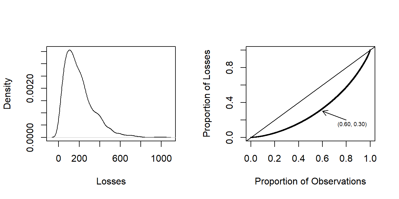
Figure 7.3: Distribution of Insurance Losses. The left-hand panel is a density plot of losses. The right-hand panel presents the same data using a Lorenz curve.
7.6.2 Performance Curve and a Gini Statistic
We now introduce a modification of the classic Lorenz curve and Gini statistic that is useful in insurance applications. Specifically, we introduce a performance curveA concentration curve is a graph of the distribution of two variables, where both variables are ordered by only one of variables. for insurance applications, it is a graph of distribution of losses versus premiums, where both losses and premiums are ordered by premiums. that, in this case, is a graph of the distribution of losses versus premiums, where both losses and premiums are ordered by premiums. To make the ideas concrete, we provide some notation and consider \(i=1, \ldots, n\) policies. For the \(i\)th policy, let
- \(y_i\) denote the insurance loss,
- \(\mathbf{x}_i\) be a set of rating variables known to the analyst, and
- \(P_i=P(\mathbf{x}_i)\) be the associated premium that is a function of \(\mathbf{x}_i\).
The set of information used to calculate the performance curve for the \(i\)th policy is \((P_i, y_i)\).
Performance Curve
It is convenient to first sort the set of policies based on premiums (from smallest to largest) and then compute the premium and loss distributions. The premium distribution is \[\begin{equation} \hat{F}_P(s) = \frac{ \sum_{i=1}^n P_i ~\mathrm{I}(P_i \leq s) }{\sum_{i=1}^n P_i} , \tag{7.5} \end{equation}\]
and the loss distribution is
\[\begin{equation} \hat{F}_{L}(s) = \frac{ \sum_{i=1}^n y_i ~\mathrm{I}(P_i \leq s) }{\sum_{i=1}^n y_i} , \tag{7.6} \end{equation}\]
where \(\mathrm{I}(\cdot)\) is the indicator function, returning a 1 if the event is true and zero otherwise. For a given value \(s\), \(\hat{F}_P(s)\) gives the proportion of premiums less than or equal to \(s\), and \(\hat{F}_{L}(s)\) gives the proportion of losses for those policyholders with premiums less than or equal to \(s\). The graph \(\left(\hat{F}_P(s),\hat{F}_{L}(s) \right)\) is known as a performance curve.
Example – Loss Distribution. Suppose we have \(n=5\) policyholders with experience as follows. The data have been ordered by premiums.
| Variable | \(i\) | 1 | 2 | 3 | 4 | 5 |
|---|---|---|---|---|---|---|
| Premium | \(P(\mathbf{x}_i)\) | 2 | 4 | 5 | 7 | 16 |
| Cumulative Premiums | \(\sum_{j=1}^i P(\mathbf{x}_j)\) | 2 | 6 | 11 | 18 | 34 |
| Loss | \(y_i\) | 2 | 5 | 6 | 6 | 17 |
| Cumulative Loss | \(\sum_{j=1}^i y_j\) | 2 | 7 | 13 | 19 | 36 |
Figure 7.4 compares the Lorenz to the performance curve. The left-hand panel shows the Lorenz curve. The horizontal axis is the cumulative proportion of policyholders (0, 0.2, 0.4, 0.6, 0.8, 1.0) and the vertical axis is the cumulative proportion of losses (0, 2/36, 7/36, 13/36, 19/39, 36/36). For the Lorenz curve, you first order by the loss size (which turns out to be the same order as premiums for this simple dataset). This figure shows a large separation between the distributions of losses and policyholders.
The right-hand panel shows the performance curve. Because observations are sorted by premiums, the first point after the origin (reading from left to right) is (2/34, 2/36). The second point is (6/34, 7/36), with the pattern continuing. From the figure, we see that there is little separation between losses and premiums.
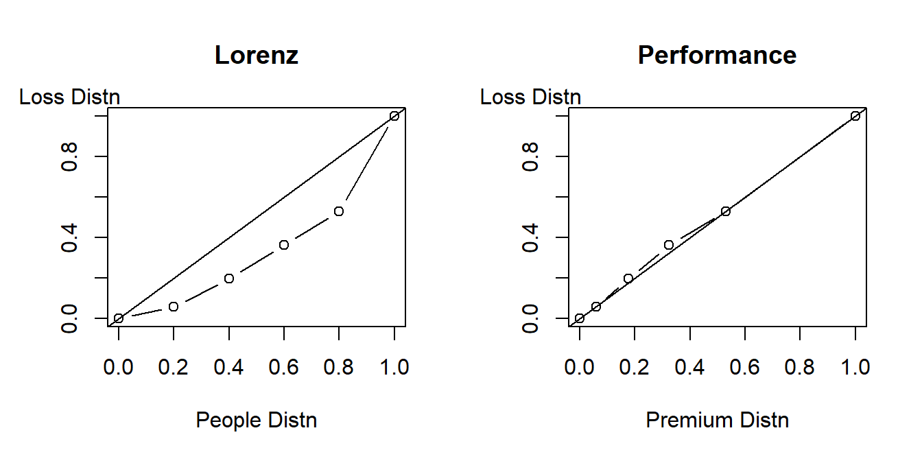
Figure 7.4: Lorenz versus Performance Curve
The performance curve can be helpful to the analyst who thinks about forming profitable portfolios for the insurer. For example, suppose that \(s\) is chosen to represent the 95th percentile of the premium distribution. Then, the horizontal axis, \(\hat{F}_P(s)\), represents the fraction of premiums for this portfolio and the vertical axis, \(\hat{F}_L(s)\), the fraction of losses for this portfolio. When developing premium principles, analysts wish to avoid unprofitable situations and make profits, or at least break even.
The expectation of the denominator in equation (7.6) is \(\sum_{i=1}^n \mathrm{E}~ [y_i]=\sum_{i=1}^n \mu_i\). Thus, if the premium principle is chosen such that \(P_i= \mu_i\), then we anticipate a close relation between the premium and loss distributions, resulting in a 45 degree line. The 45 degree line presents equality between losses and premiums, a break-even situation which is the benchmark for insurance pricing.
Gini Statistic
The classic Lorenz curve shows the proportion of policyholders on the horizontal axis and the loss distribution function on the vertical axis. The performance curve extends the classical Lorenz curve in two ways, (1) through the ordering of risks and prices by prices and (2) by allowing prices to vary by observation. We summarize the performance curve in the same way as the classic Lorenz curve using a Gini statistic, defined as twice the area between the curve and a 45 degree line. The analyst seeks ordered performance curves that approach passing through the 45 degree line; these have the least separation between the loss and premium distributions and therefore small Gini statistics.
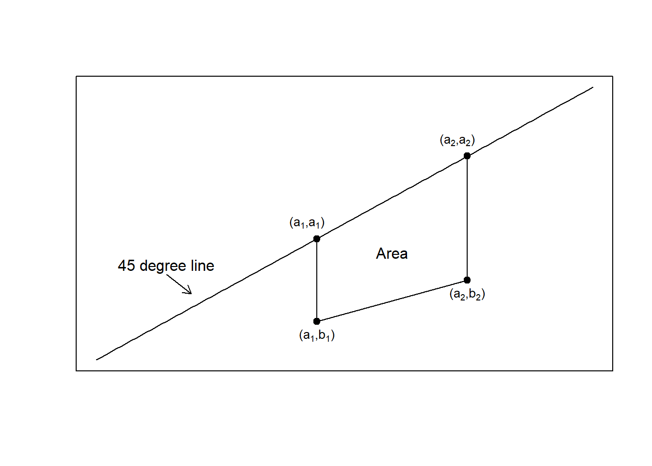
Specifically, the Gini statistic can be calculated as follows. Suppose that the empirical performance curve is given by \(\{ (a_0=0, b_0=0), (a_1, b_1), \ldots,\) \((a_n=1, b_n=1) \}\) for a sample of \(n\) observations. Here, we use \(a_j = \hat{F}_P(P_j)\) and \(b_j = \hat{F}_{L}(P_j)\). Then, the empirical Gini statistic is
\[\begin{eqnarray} \widehat{Gini} &=& 2\sum_{j=0}^{n-1} (a_{j+1} - a_j) \left \{ \frac{a_{j+1}+a_j}{2} - \frac{b_{j+1}+b_j}{2} \right\} \nonumber \\ &=& 1 - \sum_{j=0}^{n-1} (a_{j+1} - a_j) (b_{j+1}+b_j) . \tag{7.7} \end{eqnarray}\]
Show Gini Formula Details
Example – Loss Distribution: Continued. The Gini statistic for the Lorenz curve (left-hand panel of Figure 7.4) is 34.4 percent. In contrast, the Gini statistic for performance curve (right-hand panel) is 1.7 percent.
7.6.3 Out-of-Sample Validation
The benefits of out-of-sample validation for model selection were introduced in Section 4.2. We now demonstrate the use of the a Gini statistic and performance curve in this context. The procedure follows:
- Use an in-sample data set to estimate several competing models, each producing a premium function.
- Designate an out-of-sample, or validation, data set of the form \(\{(\mathbf{x}_i, y_i), i=1,\ldots,n\}\).
- Use the explanatory variables from the validation sample to form premiums of the form \(P(\mathbf{x}_i)\).
- Compute the Gini statistic for each model. Choose the model with the lowest Gini statistic.
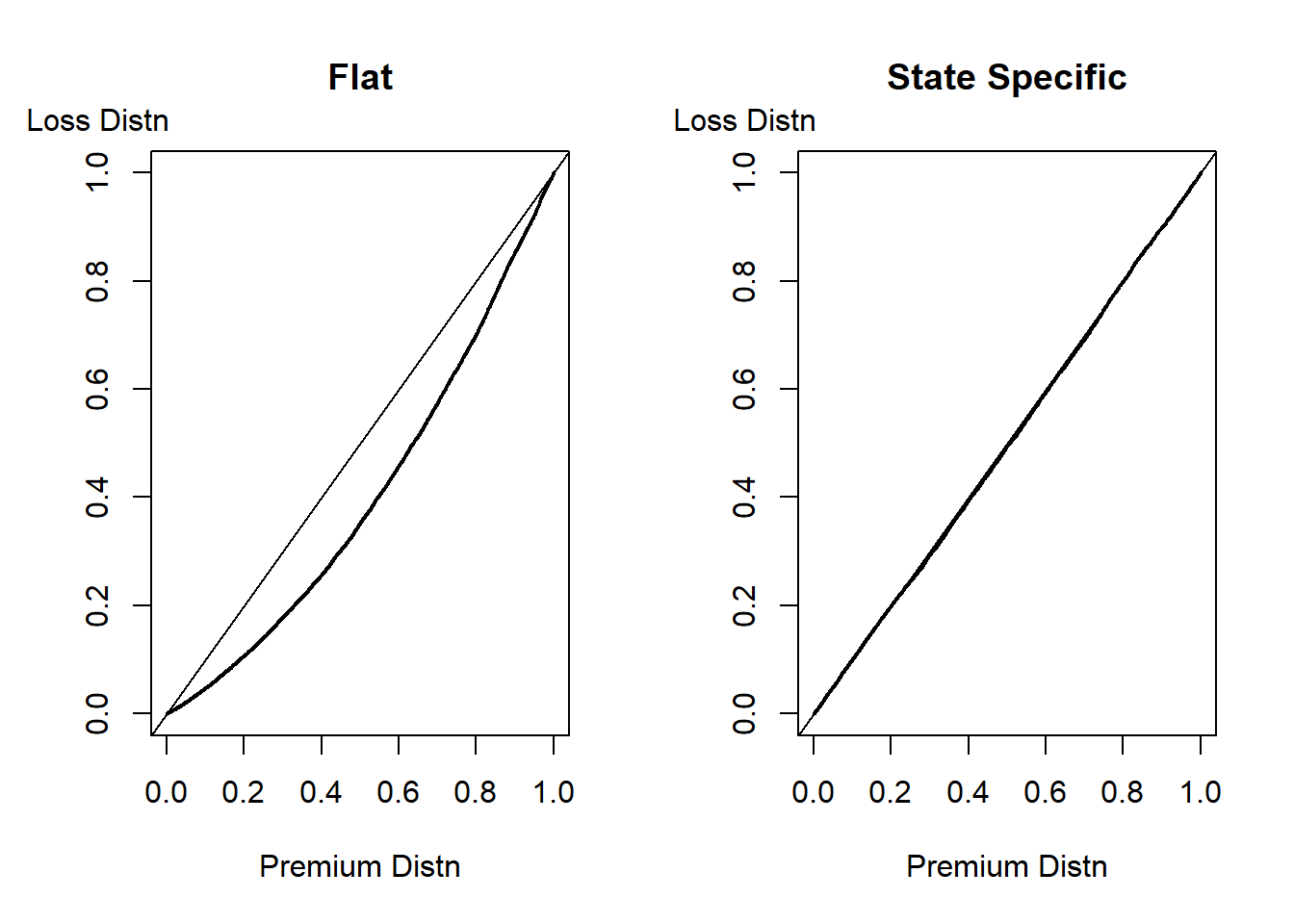
Example – Community Rating versus Premiums that Vary by State. Suppose that we have experience from 25 states and that for each state we have available 200 observations that can be used to predict future losses. For simplicity, assume that the analyst knows that these losses were generated by a gamma distribution with a common shape parameter equal to 5. Unknown to the analyst, the scale parameters vary by state from a low of 20 to 66.
- To compute base premiums, the analyst assumes a scale parameter that is common to all states that is to be estimated from the data. You can think of this common premium as based on a community ratingThis generally refers to the premium principle where all risks pay the same amount. principle.
- As an alternative, the analyst allows the scale parameters to vary by state and will again use the data to estimate these parameters.
An out of sample validation set of 100 losses from each state is available. For each of the two rating procedures, determine the performance curve and the corresponding Gini statistic. Choose the rate procedure with the lower Gini statistic.
Show Example Solution
Discussion
In insurance claims modeling, standard out-of-sample validation measures are not the most informative due to the high proportions of zeros (corresponding to no claim) and the skewed fat-tailed distribution of the positive values. In contrast, the Gini statistic works well with many zeros (see the demonstration in (Edward W. Frees, Meyers, and Cummings 2014)).
The value of the performance curves and Gini statistics have been recently advanced in the paper of Denuit, Sznajder, and Trufin (2019). Properties of an extended version, dealing with relativities for new premiums, were developed by Frees, Meyers, and Cummings (2011) and Edward W. Frees, Meyers, and Cummings (2014). In these articles you can find formulas for the standard errors and additional background information.
7.7 Further Resources and Contributors
This chapter serves as a bridge between the technical introduction of this book and an introduction to pricing and ratemaking for practicing actuaries. For readers interested in learning practical aspects of pricing, we recommend introductions by the Society of Actuaries in Friedland (2013) and by the Casualty Actuarial Society in Werner and Modlin (2016). For a classic risk management introduction to pricing, see Niehaus and Harrington (2003). See also Finger (2006) and Edward W Frees (2014).
Bühlmann (1985) was the first in the academic literature to argue that pricing should be done first at the portfolio level (he referred to this as a top down approach) which would be subsequently reconciled with pricing of individual contracts. See also the discussion in Kaas et al. (2008), Chapter 5.
For more background on pricing principles, a classic treatment is by Gerber (1979) with a more modern approach in Kaas et al. (2008). For more discussion of pricing from a financial economics viewpoint, see Bauer, Phillips, and Zanjani (2013).
- Edward W. (Jed) Frees, University of Wisconsin-Madison, and José Garrido, Concordia University are the principal authors of the initial version of this chapter. Email: jfrees@bus.wisc.edu and/or jose.garrido@concordia.ca for chapter comments and suggested improvements.
- Chapter reviewers include Chun Yong Chew, Curtis Gary Dean, Brian Hartman, and Jeffrey Pai. Write Jed or José to add you name here.
TS 7.A. Rate Regulation
Insurance regulation helps to ensure the financial stability of insurers and to protect consumers. Insurers receive premiums in return for promises to pay in the event of a contingent (insured) event. Like other financial institutions such as banks, there is a strong public interest in promoting the continuing viability of insurers.
Market Conduct
To help protect consumers, regulators impose administrative rules on the behavior of market participants. These rules, known as market conduct regulationRegulation that ensures consumers obtain fair and reasonable insurance prices and coverage, provide systems of regulatory controls that require insurers to demonstrate that they are providing fair and reliable services, including rating, in accordance with the statutes and regulations of a jurisdiction.
- Product regulation serves to protect consumers by ensuring that insurance policy provisions are reasonable and fair, and do not contain major gaps in coverage that might be misunderstood by consumers and leave them unprotected.
- The insurance product is the insurance contract (policy) and the coverage it provides. Insurance contracts are regulated for these reasons:
- Insurance policies are complex legal documents that are often difficult to interpret and understand.
- Insurers write insurance policies and sell them to the public on a “take it or leave it” basis.
Market conduct includes rules for intermediaries such as agents (who sell insurance to individuals) and brokers (who sell insurance to businesses). Market conduct also includes competition policy regulation, designed to ensure an efficient and competitive marketplace that offers low prices to consumers.
Rate Regulation
Rate regulation helps guide the development of premiums and so is the focus of this chapter. As with other aspects of market conduct regulation, the intent of these regulations is to ensure that insurers not take unfair advantage of consumers. Rate (and policy form) regulation is common worldwide.
The amount of regulatory scrutiny varies by insurance product. Rate regulation is uncommon in life insurance. Further, in non-life insurance, most commercial lines and reinsurance are free from regulation. Rate regulation is common in automobile insurance, health insurance, workers compensation, medical malpractice, and homeowners insurance. These are markets in which insurance is mandatory or in which universal coverage is thought to be socially desirable.
There are three principles that guide rate regulation: rates should
- be adequate (to maintain insurance company solvency),
- but not excessive (not so high as to lead to exorbitant profits),
- nor unfairly discriminatory (price differences must reflect expected claim and expense differences).
Recently, in auto and home insurance, the twin issues of availability and affordability, which are not explicitly included in the guiding principles, have been assuming greater importance in regulatory decisions.
Rates are Not Unfairly Discriminatory
Some government regulations of insurance restrict the amount, or level, of premium rates. These are based on the first two of the three guiding rate regulation principles, that rates be adequate but not excessive. This type of regulation is discussed further in the following section on types of rate regulation.
Other government regulations restrict the type of information that can be used in risk classification. These are based on the third guiding principle, that rates not be unfairly discriminatory. “Discrimination” in an insurance context has a different meaning than commonly used; for our purposes, discrimination means the ability to distinguish among things or, in our case, policyholders. The real issue is what is meant by the adjective “fair.”
In life insurance, it has long been held that it is reasonable and fair to charge different premium rates by age. For example, a life insurance premium differs dramatically between an 80 year old and someone aged 20. In contrast, it is unheard of to use rates that differ by:
- ethnicity or race,
- political affiliation, or
- religion.
It is not a matter of whether data can be used to establish statistical significance among the levels of any of these variables. Rather, it is a societal decision as to what constitutes notions of “fairness.”
Different jurisdictions have taken different stances on what constitutes a fair rating variable. For example, in some jurisdictions for some insurance products, gender is no longer a permissible variable. As an illustration, the European Union now prohibits the use of gender for automobile rating. As another example, in the U.S., many discussions have revolved around the use of credit ratings to be used in automobile insurance pricing. Credit ratings are designed to measure consumer financial responsibility. Yet, some argue that credit scores are good proxies for ethnicity and hence should be prohibited.
In an age where more data is being used in imaginative ways, discussions of what constitutes a fair rating variable will only become more important going forward and much of that discussion is beyond the scope of this text. However, it is relevant to the discussion to remark that actuaries and other data analysts can contribute to societal discussions on what constitutes a “fair” rating variable in unique ways by establishing the magnitude of price differences when using variables under discussion.
Types of Rate Regulation
There are several methods, that vary by the level of scrutiny, by which regulators may restrict the rates that insurers offer.
The most restrictive is a government prescribedGovernment sets the entire rating system including coverages regulatory system, where the government regulator determines and promulgates the rates, classifications, forms, and so forth, to which all insurers must adhere. Also restrictive are prior approvalRegulator must approve rates, forms, rules filed by insurers before use systems. Here, the insurer must file rates, rules, and so forth, with government regulators. Depending on the statute, the filing becomes effective when a specified waiting period elapses (if the government regulator does not take specific action on the filing, it is deemed approved automatically) or when the government regulator formally approves the filing.
The least restrictive is a no fileInsurers may use new rates, forms, rules without approval from regulators or record maintenance system where the insurer need not file rates, rules, and so forth, with the government regulator. The regulator may periodically examine the insurer to ensure compliance with the law. Another relatively flexible system is the file onlyInsurers must file rates, forms, rules for record keeping and use immediately system, also known as competitive rating, where the insurer simply keeps files to ensure compliance with the law.
In between these two extremes are the (1) file and use, (2) use and file, (3) modified prior approval, and (4) flex rating systems.
- File and Use: The insurer must file rates, rules, and so forth, with the government regulator. The filing becomes effective immediately or on a future date specified by the filer.
- Use and File: The filing becomes effective when used. The insurer must file rates, rules, and so forth, with the government regulator within a specified time period after first use.
- Modified Prior Approval: This is a hybrid of “prior approval” and “file and use” laws. If the rate revision is based solely on a change in loss experience then “file and use” may apply. However, if the rate revision is based on a change in expense relationships or rate classifications, then “prior approval” may apply.
- Flex (or Band) Rating: The insurer may increase or decrease a rate within a “flex band,” or range, without approval of the government regulator. Generally, either “file and use” or “use and file” provisions apply.
For a broad introduction to government insurance regulation from a global perspective, see the website of the International Association of Insurance Supervisors (IAIS).
Bibliography
Bauer, Daniel, Richard D. Phillips, and George H. Zanjani. 2013. “Financial Pricing of Insurance.” In Handbook of Insurance, 627–45. Springer.
Denuit, Michel, Dominik Sznajder, and Julien Trufin. 2019. “Model Selection Based on Lorenz and Concentration Curves, Gini Indices and Convex Order.” Insurance: Mathematics and Economics.
Finger, Robert J. 2006. “Risk Classification.” In Foundations of Casualty Actuarial Science, 231–76.
Frees, Edward W. 2014. “Frequency and Severity Models.” In Predictive Modeling Applications in Actuarial Science, edited by Edward W Frees, Glenn Meyers, and Richard Derrig, 1:138–64. Cambridge University Press Cambridge.
Frees, Edward W., Glenn Meyers, and A. David Cummings. 2011. “Summarizing Insurance Scores Using a Gini Index.” Journal of the American Statistical Association 106 (495): 1085–98.
Frees, Edward W., Glenn Meyers, and A. David Cummings. 2011. “Summarizing Insurance Scores Using a Gini Index.” Journal of the American Statistical Association 106 (495): 1085–98.
2014. “Insurance Ratemaking and a Gini Index.” Journal of Risk and Insurance 81 (2): 335–66.Friedland, Jacqueline. 2013. Fundamentals of General Insurance Actuarial Analysis. Society of Actuaries.
Gerber, Hans U. 1979. An Introduction to Mathematical Risk Theory, Vol. 8 of Ss Heubner Foundation Monograph Series. University of Pennsylvania Wharton School SS Huebner Foundation for Insurance Education.
Kaas, Rob, Marc Goovaerts, Jan Dhaene, and Michel Denuit. 2008. Modern Actuarial Risk Theory: Using R. Vol. 128. Springer Science & Business Media.
Lorenz, Max O. 1905. “Methods of Measuring the Concentration of Wealth.” Publications of the American Statistical Association 9 (70): 209–19.
Niehaus, Gregory, and Scott Harrington. 2003. Risk Management and Insurance. New York: McGraw Hill.
Werner, Geoff, and Claudine Modlin. 2016. Basic Ratemaking, Fifth Edition. Casualty Actuarial Society. https://www.casact.org/library/studynotes/werner_modlin_ratemaking.pdf.