Chapter 15 Appendix A: Review of Statistical Inference

Chapter Preview. The appendix gives an overview of concepts and methods related to statistical inference on the population of interest, using a random sample of observations from the population. In the appendix, Section 15.1 introduces the basic concepts related to the population and the sample used for making the inference. Section 15.2 presents the commonly used methods for point estimation of population characteristics. Section 15.3 demonstrates interval estimation that takes into consideration the uncertainty in the estimation, due to use of a random sample from the population. Section 15.4 introduces the concept of hypothesis testing for the purpose of variable and model selection.

15.1 Basic Concepts

---

In this section, you learn the following concepts related to statistical inference.

• Random sampling from a population that can be summarized using a list of items or individuals within the population
• Sampling distributions that characterize the distributions of possible outcomes for a statistic calculated from a random sample
• The central limit theorem that guides the distribution of the mean of a random sample from the population

---

Statistical inference is the process of making conclusions on the characteristics of a large set of items/individuals (i.e., the population), using a representative set of data (e.g., a random sample) from a list of items or individuals from the population that can be sampled. While the process has a broad spectrum of applications in various areas including science, engineering, health, social, and economic fields, statistical inference is important to insurance companies that use data from their existing policy holders in order to make inference on the characteristics (e.g., risk profiles) of a specific segment of target customers (i.e., the population) whom the insurance companies do not directly observe.

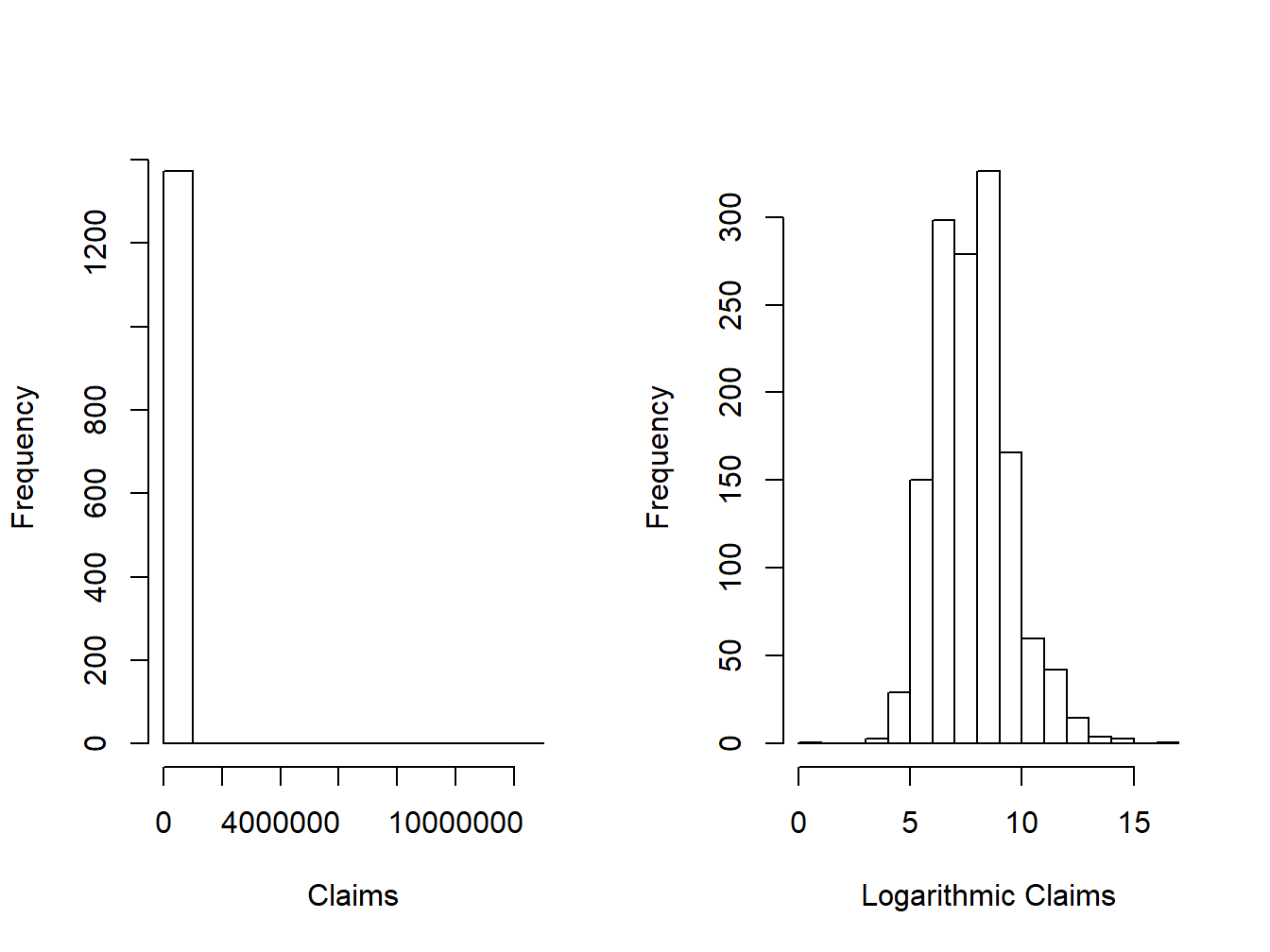
Show An Empirical Example Using the Wisconsin Property Fund

Example – Wisconsin Property Fund. Assume there are 1,377 individual claims from the 2010 experience.

	Minimum	First Quartile	Median	Mean	Third Quartile	Maximum	Standard Deviation
Claims	1	788	2,250	26,620	6,171	12,920,000	368,030
Logarithmic Claims	0	6.670	7.719	7.804	8.728	16.370	1.683

ClaimLev <- read.csv("Data/CLAIMLEVEL.csv", header=TRUE)
ClaimLevBC10<-subset(ClaimLev,Year==2010); 
cat("Sample size: ", nrow(ClaimLevBC10), "\n")
par(mfrow=c(1, 2))
hist(ClaimLevBC10$Claim, main="", xlab="Claims")
hist(log(ClaimLevBC10$Claim), main="", xlab="Logarithmic Claims")

Figure 15.1: Distribution of Claims

## Sample size:  1377

Using the 2010 claim experience (the sample), the Wisconsin Property Fund may be interested in assessing the severity of all claims that could potentially occur, such as 2010, 2011, and so forth (the population). This process is important in the contexts of ratemaking or claim predictive modeling. In order for such inference to be valid, we need to assume that

• the set of 2010 claims is a random sample that is representative of the population,
• the sampling distribution of the average claim amount can be estimated, so that we can quantify the bias and uncertainty in the estimation due to use of a finite sample.

15.1.1 Random Sampling

In statistics, a sampling error occurs when the sampling frame, the list from which the sample is drawn, is not an adequate approximation of the population of interest. A sample must be a representative subset of a population, or universe, of interest. If the sample is not representative, taking a larger sample does not eliminate bias, as the same mistake is repeated over again and again. Thus, we introduce the concept for random sampling that gives rise to a simple random sample that is representative of the population.

We assume that the random variable \(X\) represents a draw from a population with a distribution function \(F(\cdot)\) with mean \(\mathrm{E}[X]=\mu\) and variance \(\mathrm{Var}[X]=\mathrm{E}[(X-\mu)^2]\), where \(E(\cdot)\) denotes the expectation of a random variable. In random sampling, we make a total of \(n\) such draws represented by \(X_1, \ldots, X_n\), each unrelated to one another (i.e., statistically independent). We refer to \(X_1, \ldots, X_n\) as a random sample (with replacement) from \(F(\cdot)\), taking either a parametric or nonparametric form. Alternatively, we may say that \(X_1, \ldots, X_n\) are identically and independently distributed (iid) with distribution function \(F(\cdot)\).

15.1.2 Sampling Distribution

Using the random sample \(X_1, \ldots, X_n\), we are interested in making a conclusion on a specific attribute of the population distribution \(F(\cdot)\). For example, we may be interested in making an inference on the population mean, denoted \(\mu\). It is natural to think of the sample mean, \(\bar{X}=\sum_{i=1}^nX_i\), as an estimate of the population mean \(\mu\). We call the sample mean as a statistic calculated from the random sample \(X_1, \ldots, X_n\). Other commonly used summary statistics include sample standard deviation and sample quantiles.

When using a statistic (e.g., the sample mean \(\bar{X}\)) to make statistical inference on the population attribute (e.g., population mean \(\mu\)), the quality of inference is determined by the bias and uncertainty in the estimation, owing to the use of a sample in place of the population. Hence, it is important to study the distribution of a statistic that quantifies the bias and variability of the statistic. In particular, the distribution of the sample mean, \(\bar{X}\) (or any other statistic), is called the sampling distribution. The sampling distribution depends on the sampling process, the statistic, the sample size \(n\) and the population distribution \(F(\cdot)\). The central limit theorem gives the large-sample (sampling) distribution of the sample mean under certain conditions.

15.1.3 Central Limit Theorem

In statistics, there are variations of the central limit theorem (CLT) ensuring that, under certain conditions, the sample mean will approach the population mean with its sampling distribution approaching the normal distribution as the sample size goes to infinity. We give the Lindeberg–Levy CLT that establishes the asymptotic sampling distribution of the sample mean \(\bar{X}\) calculated using a random sample from a universe population having a distribution \(F(\cdot)\).

Lindeberg–Levy CLT. Let \(X_1, \ldots, X_n\) be a random sample from a population distribution \(F(\cdot)\) with mean \(\mu\) and variance \(\sigma^2<\infty\). The difference between the sample mean \(\bar{X}\) and \(\mu\), when multiplied by \(\sqrt{n}\), converges in distribution to a normal distribution as the sample size goes to infinity. That is, \[\sqrt{n}(\bar{X}-\mu)\xrightarrow[]{d}N(0,\sigma).\]

Note that the CLT does not require a parametric form for \(F(\cdot)\). Based on the CLT, we may perform statistical inference on the population mean (we infer, not deduce). The types of inference we may perform include estimation of the population, hypothesis testing on whether a null statement is true, and prediction of future samples from the population.

15.2 Point Estimation and Properties

---

In this section, you learn how to

• estimate population parameters using method of moments estimation
• estimate population parameters based on maximum likelihood estimation

---

The population distribution function \(F(\cdot)\) can usually be characterized by a limited (finite) number of terms called parameters, in which case we refer to the distribution as a parametric distribution. In contrast, in nonparametric analysis, the attributes of the sampling distribution are not limited to a small number of parameters.

For obtaining the population characteristics, there are different attributes related to the population distribution \(F(\cdot)\). Such measures include the mean, median, percentiles (i.e., 95th percentile), and standard deviation. Because these summary measures do not depend on a specific parametric reference, they are nonparametric summary measures.

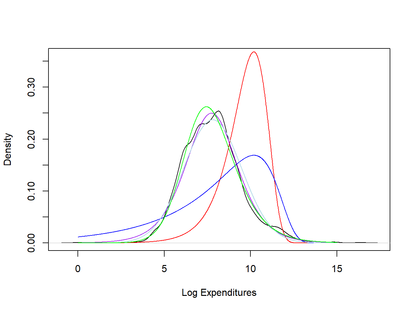
In parametric analysis, on the other hand, we may assume specific families of distributions with specific parameters. For example, people usually think of logarithm of claim amounts to be normally distributed with mean \(\mu\) and standard deviation \(\sigma\). That is, we assume that the claims have a lognormal distribution with parameters \(\mu\) and \(\sigma\). Alternatively, insurance companies commonly assume that claim severity follows a gamma distribution with a shape parameter \(\alpha\) and a scale parameter \(\theta\). Here, the normal, lognormal, and gamma distributions are examples of parametric distributions. In the above examples, the quantities of \(\mu\), \(\sigma\), \(\alpha\), and \(\theta\) are known as parameters. For a given parametric distribution family, the distribution is uniquely determined by the values of the parameters.

One often uses \(\theta\) to denote a summary attribute of the population. In parametric models, \(\theta\) can be a parameter or a function of parameters from a distribution such as the normal mean and variance parameters. In nonparametric analysis, it can take a form of a nonparametric summary such as the population mean or standard deviation. Let \(\hat{\theta} =\hat{\theta}(X_1, \ldots, X_n)\) be a function of the sample that provides a proxy, or an estimate, of \(\theta\). It is referred to as a statistic, a function of the sample \(X_1, \ldots, X_n\).

Show Wisconsin Property Fund Example - Continued

Example – Wisconsin Property Fund. The sample mean 7.804 and the sample standard deviation 1.683 can be either deemed as nonparametric estimates of the population mean and standard deviation, or as parametric estimates of \(\mu\) and \(\sigma\) of the normal distribution concerning the logarithmic claims. Using results from the lognormal distribution, we may estimate the expected claim, the lognormal mean, as 10,106.8 ( \(=\exp(7.804+1.683^2/2)\) ).

For the Wisconsin Property Fund data, we may denote \(\hat{\mu} =7.804\) and \(\hat{\sigma} = 1.683\), with the hat notation denoting an estimate of the parameter based on the sample. In particular, such an estimate is referred to as a point estimate, a single approximation of the corresponding parameter. For point estimation, we introduce the two commonly used methods called the method of moments estimation and maximum likelihood estimation.

15.2.1 Method of Moments Estimation

Before defining the method of moments estimation, we define the the concept of moments. Moments are population attributes that characterize the distribution function \(F(\cdot)\). Given a random draw \(X\) from \(F(\cdot)\), the expectation \(\mu_k=\mathrm{E}[X^k]\) is called the \(k\)th moment of \(X\), \(k=1,2,3,\ldots\) For example, the population mean \(\mu\) is the first moment. Furthermore, the expectation \(\mathrm{E}[(X-\mu)^k]\) is called a \(k\)th central moment. Thus, the variance is the second central moment.

Using the random sample \(X_1, \ldots, X_n\), we may construct the corresponding sample moment, \(\hat{\mu}_k=(1/n)\sum_{i=1}^n X_i^k\), for estimating the population attribute \(\mu_k\). For example, we have used the sample mean \(\bar{X}\) as an estimator for the population mean \(\mu\). Similarly, the second central moment can be estimated as \((1/n)\sum_{i=1}^n(X_i-\bar{X})^2\). Without assuming a parametric form for \(F(\cdot)\), the sample moments constitute nonparametric estimates of the corresponding population attributes. Such an estimator based on matching of the corresponding sample and population moments is called a method of moments estimator (mme).

While the mme works naturally in a nonparametric model, it can be used to estimate parameters when a specific parametric family of distribution is assumed for \(F(\cdot)\). Denote by \(\boldsymbol{\theta}=(\theta_1,\cdots,\theta_m)\) the vector of parameters corresponding to a parametric distribution \(F(\cdot)\). Given a distribution family, we commonly know the relationships between the parameters and the moments. In particular, we know the specific forms of the functions \(h_1(\cdot),h_2(\cdot),\cdots,h_m(\cdot)\) such that \(\mu_1=h_1(\boldsymbol{\theta}),\,\mu_2=h_2(\boldsymbol{\theta}),\,\cdots,\,\mu_m=h_m(\boldsymbol{\theta})\). Given the mme \(\hat{\mu}_1, \ldots, \hat{\mu}_m\) from the random sample, the mme of the parameters \(\hat{\theta}_1,\cdots,\hat{\theta}_m\) can be obtained by solving the equations of \[\hat{\mu}_1=h_1(\hat{\theta}_1,\cdots,\hat{\theta}_m);\] \[\hat{\mu}_2=h_2(\hat{\theta}_1,\cdots,\hat{\theta}_m);\] \[\cdots\] \[\hat{\mu}_m=h_m(\hat{\theta}_1,\cdots,\hat{\theta}_m).\]

Show Wisconsin Property Fund Example - Continued

Example – Wisconsin Property Fund. Assume that the claims follow a lognormal distribution, so that logarithmic claims follow a normal distribution. Specifically, assume \(\log(X)\) has a normal distribution with mean \(\mu\) and variance \(\sigma^2\), denoted as \(\log(X) \sim N(\mu, \sigma^2)\). It is straightforward that the mme \(\hat{\mu}=\bar{X}\) and \(\hat{\sigma}=\sqrt{(1/n)\sum_{i=1}^n(X_i-\bar{X})^2}\). For the Wisconsin Property Fund example, the method of moments estimates are \(\hat{\mu} =7.804\) and \(\hat{\sigma} = 1.683\).

15.2.2 Maximum Likelihood Estimation

When \(F(\cdot)\) takes a parametric form, the maximum likelihood method is widely used for estimating the population parameters \(\boldsymbol{\theta}\). Maximum likelihood estimation is based on the likelihood function, a function of the parameters given the observed sample. Denote by \(f(x_i|\boldsymbol{\theta})\) the probability function of \(X_i\) evaluated at \(X_i=x_i\) \((i=1,2,\cdots,n)\); it is the probability mass function in the case of a discrete \(X\) and the probability density function in the case of a continuous \(X\). Assuming independence, the likelihood function of \(\boldsymbol{\theta}\) associated with the observation \((X_1,X_2,\cdots,X_n)=(x_1,x_2,\cdots,x_n)=\mathbf{x}\) can be written as \[L(\boldsymbol{\theta}|\mathbf{x})=\prod_{i=1}^nf(x_i|\boldsymbol{\theta}),\] with the corresponding log-likelihood function given by \[l(\boldsymbol{\theta}|\mathbf{x})=\log(L(\boldsymbol{\theta}|\mathbf{x}))=\sum_{i=1}^n\log f(x_i|\boldsymbol{\theta}).\] The maximum likelihood estimator (mle) of \(\boldsymbol{\theta}\) is the set of values of \(\boldsymbol{\theta}\) that maximize the likelihood function (log-likelihood function), given the observed sample. That is, the mle \(\hat{\boldsymbol{\theta}}\) can be written as \[\hat{\boldsymbol{\theta}}={\mbox{argmax}}_{\boldsymbol{\theta}\in\Theta}l(\boldsymbol{\theta}|\mathbf{x}),\] where \(\Theta\) is the parameter space of \(\boldsymbol{\theta}\), and \({\mbox{argmax}}_{\boldsymbol{\theta}\in\Theta}l(\boldsymbol{\theta}|\mathbf{x})\) is defined as the value of \(\boldsymbol{\theta}\) at which the function \(l(\boldsymbol{\theta}|\mathbf{x})\) reaches its maximum.

Given the analytical form of the likelihood function, the mle can be obtained by taking the first derivative of the log-likelihood function with respect to \(\boldsymbol{\theta}\), and setting the values of the partial derivatives to zero. That is, the mle are the solutions of the equations of \[\frac{\partial l(\hat{\boldsymbol{\theta}}|\mathbf{x})}{\partial\hat{\theta}_1}=0;\] \[\frac{\partial l(\hat{\boldsymbol{\theta}}|\mathbf{x})}{\partial\hat{\theta}_2}=0;\] \[\cdots\] \[\frac{\partial l(\hat{\boldsymbol{\theta}}|\mathbf{x})}{\partial\hat{\theta}_m}=0,\] provided that the second partial derivatives are negative.

For parametric models, the mle of the parameters can be obtained either analytically (e.g., in the case of normal distributions and linear estimators), or numerically through iterative algorithms such as the Newton-Raphson method and its adaptive versions (e.g., in the case of generalized linear models with a non-normal response variable).

Normal distribution. Assume \((X_1,X_2,\cdots,X_n)\) to be a random sample from the normal distribution \(N(\mu, \sigma^2)\). With an observed sample \((X_1,X_2,\cdots,X_n)=(x_1,x_2,\cdots,x_n)\), we can write the likelihood function of \(\mu,\sigma^2\) as \[L(\mu,\sigma^2)=\prod_{i=1}^n\left[\frac{1}{\sqrt{2\pi\sigma^2}}e^{-\frac{\left(x_i-\mu\right)^2}{2\sigma^2}}\right],\] with the corresponding log-likelihood function given by \[l(\mu,\sigma^2)=-\frac{n}{2}[\log(2\pi)+\log(\sigma^2)]-\frac{1}{2\sigma^2}\sum_{i=1}^n\left(x_i-\mu\right)^2.\]

By solving \[\frac{\partial l(\hat{\mu},\sigma^2)}{\partial \hat{\mu}}=0,\] we obtain \(\hat{\mu}=\bar{x}=(1/n)\sum_{i=1}^nx_i\). It is straightforward to verify that \(\frac{\partial l^2(\hat{\mu},\sigma^2)}{\partial \hat{\mu}^2}\left|_{\hat{\mu}=\bar{x}}\right.<0\). Since this works for arbitrary \(x\), \(\hat{\mu}=\bar{X}\) is the mle of \(\mu\). Similarly, by solving \[\frac{\partial l(\mu,\hat{\sigma}^2)}{\partial \hat{\sigma}^2}=0,\] we obtain \(\hat{\sigma}^2=(1/n)\sum_{i=1}^n(x_i-\mu)^2\). Further replacing \(\mu\) by \(\hat{\mu}\), we derive the mle of \(\sigma^2\) as \(\hat{\sigma}^2=(1/n)\sum_{i=1}^n(X_i-\bar{X})^2\).

Hence, the sample mean \(\bar{X}\) and \(\hat{\sigma}^2\) are both the mme and MLEMaximum likelihood estimate for the mean \(\mu\) and variance \(\sigma^2\), under a normal population distribution \(F(\cdot)\). More details regarding the properties of the likelihood function are given in Appendix Section 17.1.

15.3 Interval Estimation

---

In this section, you learn how to

• derive the exact sampling distribution of the mle of the normal mean
• obtain the large-sample approximation of the sampling distribution using the large sample properties of the mle
• construct a confidence interval of a parameter based on the large sample properties of the mle

---

Now that we have introduced the mme and mle, we may perform the first type of statistical inference, interval estimation that quantifies the uncertainty resulting from the use of a finite sample. By deriving the sampling distribution of mle, we can estimate an interval (a confidence interval) for the parameter. Under the frequentist approach (e.g., that based on maximum likelihood estimation), the confidence intervals generated from the same random sampling frame will cover the true value the majority of times (e.g., 95% of the times), if we repeat the sampling process and re-calculate the interval over and over again. Such a process requires the derivation of the sampling distribution for the mle.

15.3.1 Exact Distribution for Normal Sample Mean

Due to the additivity property of the normal distribution (i.e., a sum of normal random variables that follows a multivariate normal distribution still follows a normal distribution) and that the normal distribution belongs to the location–scale family (i.e., a location and/or scale transformation of a normal random variable has a normal distribution), the sample mean \(\bar{X}\) of a random sample from a normal \(F(\cdot)\) has a normal sampling distribution for any finite \(n\). Given \(X_i\sim^{iid} N(\mu,\sigma^2)\), \(i=1,\dots,n\), the mle of \(\mu\) has an exact distribution \[\bar{X}\sim N\left(\mu,\frac{\sigma^2}{n}\right).\] Hence, the sample mean is an unbiased estimator of \(\mu\). In addition, the uncertainty in the estimation can be quantified by its variance \(\sigma^2/n\), that decreases with the sample size \(n\). When the sample size goes to infinity, the sample mean will approach a single mass at the true value.

15.3.2 Large-sample Properties of MLE

For the mle of the mean parameter and any other parameters of other parametric distribution families, however, we usually cannot derive an exact sampling distribution for finite samples. Fortunately, when the sample size is sufficiently large, mles can be approximated by a normal distribution. Due to the general maximum likelihood theory, the mle has some nice large-sample properties.

• The mle \(\hat{\theta}\) of a parameter \(\theta\), is a consistent estimator. That is, \(\hat{\theta}\) converges in probability to the true value \(\theta\), as the sample size \(n\) goes to infinity.

• The mle has the asymptotic normality property, meaning that the estimator will converge in distribution to a normal distribution centered around the true value, when the sample size goes to infinity. Namely, \[\sqrt{n}(\hat{\theta}-\theta)\rightarrow_d N\left(0,\,V\right),\quad \mbox{as}\quad n\rightarrow \infty,\] where \(V\) is the inverse of the Fisher Information. Hence, the mle \(\hat{\theta}\) approximately follows a normal distribution with mean \(\theta\) and variance \(V/n\), when the sample size is large.

• The mle is efficient, meaning that it has the smallest asymptotic variance \(V\), commonly referred to as the Cramer–Rao lower bound. In particular, the Cramer–Rao lower bound is the inverse of the Fisher information defined as \(\mathcal{I}(\theta)=-\mathrm{E}(\partial^2\log f(X;\theta)/\partial \theta^2)\). Hence, \(\mathrm{Var}(\hat{\theta})\) can be estimated based on the observed Fisher information that can be written as \(-\sum_{i=1}^n \partial^2\log f(X_i;\theta)/\partial \theta^2\).

For many parametric distributions, the Fisher information may be derived analytically for the mle of parameters. For more sophisticated parametric models, the Fisher information can be evaluated numerically using numerical integration for continuous distributions, or numerical summation for discrete distributions. More details regarding maximum likelihood estimation are given in Appendix Section 17.2.

15.3.3 Confidence Interval

Given that the mle \(\hat{\theta}\) has either an exact or an approximate normal distribution with mean \(\theta\) and variance \(\mathrm{Var}(\hat{\theta})\), we may take the square root of the variance and plug-in the estimate to define \(se(\hat{\theta}) = \sqrt{\mathrm{Var}(\hat{\theta})}\). A standard error is an estimated standard deviation that quantifies the uncertainty in the estimation resulting from the use of a finite sample. Under some regularity conditions governing the population distribution, we may establish that the statistic

\[ \frac{\hat{\theta}-\theta}{se(\hat{\theta})} \]

converges in distribution to a Student-\(t\) distribution with degrees of freedom (a parameter of the distribution) \({n-p}\), where \(p\) is the number of parameters in the model other than the variance. For example, for the normal distribution case, we have \(p=1\) for the parameter \(\mu\); for a linear regression model with an independent variable, we have \(p=2\) for the parameters of the intercept and the independent variable. Denote by \(t_{n-p}(1-\alpha/2)\) the \(100\times(1-\alpha/2)\)-th percentile of the Student-\(t\) distribution that satisfies \(\Pr\left[t< t_{n-p}\left(1-{\alpha}/{2}\right) \right]= 1-{\alpha}/{2}\). We have,

\[ \Pr\left[-t_{n-p}\left(1-\frac{\alpha}{2}\right)<\frac{\hat{\theta}-\theta}{se(\hat{\theta})}< t_{n-p}\left(1-\frac{\alpha}{2}\right) \right]= 1-{\alpha}, \]

from which we can derive a confidence interval for \(\theta\). From the above equation we can derive a pair of statistics, \(\hat{\theta}_1\) and \(\hat{\theta}_2\), that provide an interval of the form \([\hat{\theta}_1, \hat{\theta}_2]\). This interval is a \(1-\alpha\) confidence interval for \(\theta\) such that \(\Pr\left(\hat{\theta}_1 \le \theta \le \hat{\theta}_2\right) = 1-\alpha,\) where the probability \(1-\alpha\) is referred to as the confidence level. Note that the above confidence interval is not valid for small samples, except for the case of the normal mean.

Normal distribution. For the normal population mean \(\mu\), the mle has an exact sampling distribution \(\bar{X}\sim N(\mu,\sigma/\sqrt{n})\), in which we can estimate \(se(\hat{\theta})\) by \(\hat{\sigma}/\sqrt{n}\). Based on the Cochran’s theorem, the resulting statistic has an exact Student-\(t\) distribution with degrees of freedom \(n-1\). Hence, we can derive the lower and upper bounds of the confidence interval as

\[ \hat{\mu}_1 = \hat{\mu} - t_{n-1}\left(1-\frac{\alpha}{2}\right)\frac{ \hat{\sigma}}{\sqrt{n}} \]

and

\[ \hat{\mu}_2 = \hat{\mu} + t_{n-1}\left(1-\frac{\alpha}{2}\right)\frac{ \hat{\sigma}}{\sqrt{n}}. \]

When \(\alpha = 0.05\), \(t_{n-1}(1-\alpha/2) \approx 1.96\) for large values of \(n\). Based on the Cochran’s theorem, the confidence interval is valid regardless of the sample size.

---

Show Wisconsin Property Fund Example - Continued

Example – Wisconsin Property Fund. For the lognormal claim model, (7.715235, 7.893208) is a 95% confidence interval for \(\mu\).

More details regarding interval estimation based the mle of other parameters and distribution families are given in Appendix Chapter 17.

---

15.4 Hypothesis Testing

---

In this section, you learn how to

• understand the basic concepts in hypothesis testing including the level of significance and the power of a test
• perform hypothesis testing such as a Student-\(t\) test based on the properties of the mle
• construct a likelihood ratio test for a single parameter or multiple parameters from the same statistical model
• use information criteria such as the Akaike’s information criterion or the Bayesian information criterion to perform model selection

---

For the parameter(s) \(\boldsymbol{\theta}\) from a parametric distribution, an alternative type of statistical inference is called hypothesis testing that verifies whether a hypothesis regarding the parameter(s) is true, under a given probability called the level of significance \(\alpha\) (e.g., 5%). In hypothesis testing, we reject the null hypothesis, a restrictive statement concerning the parameter(s), if the probability of observing a random sample as extremal as the observed one is smaller than \(\alpha\), if the null hypothesis were true.

15.4.1 Basic Concepts

In a statistical test, we are usually interested in testing whether a statement regarding some parameter(s), a null hypothesis (denoted \(H_0\)), is true given the observed data. The null hypothesis can take a general form \(H_0:\theta\in\Theta_0\), where \(\Theta_0\) is a subset of the parameter space \(\Theta\) of \(\theta\) that may contain multiple parameters. For the case with a single parameter \(\theta\), the null hypothesis usually takes either the form \(H_0:\theta=\theta_0\) or \(H_0:\theta\leq\theta_0\). The opposite of the null hypothesis is called the alternative hypothesis that can be written as \(H_a:\theta\neq\theta_0\) or \(H_a:\theta>\theta_0\). The statistical test on \(H_0:\theta=\theta_0\) is called a two-sided as the alternative hypothesis contains two inequalities of \(H_a:\theta<\theta_0\) or \(\theta>\theta_0\). In contrast, the statistical test on either \(H_0:\theta\leq\theta_0\) or \(H_0:\theta\geq\theta_0\) is called a one-sided test.

A statistical test is usually constructed based on a statistic \(T\) and its exact or large-sample distribution. The test typically rejects a two-sided test when either \(T > c_1\) or \(T < c_2\), where the two constants \(c_1\) and \(c_2\) are obtained based on the sampling distribution of \(T\) at a probability level \(\alpha\) called the level of significance. In particular, the level of significance \(\alpha\) satisfies

\[ \alpha=\Pr(\mbox{reject }H_0|H_0\mbox{ is true}), \]

meaning that if the null hypothesis were true, we would reject the null hypothesis only 5% of the times, if we repeat the sampling process and perform the test over and over again.

Thus, the level of significance is the probability of making a type I error (error of the first kind), the error of incorrectly rejecting a true null hypothesis. For this reason, the level of significance \(\alpha\) is also referred to as the type I error rate. Another type of error we may make in hypothesis testing is the type II error (error of the second kind), the error of incorrectly accepting a false null hypothesis. Similarly, we can define the type II error rate as the probability of not rejecting (accepting) a null hypothesis given that it is not true. That is, the type II error rate is given by

\[ \Pr(\mbox{accept }H_0|H_0\mbox{ is false}). \]

Another important quantity concerning the quality of the statistical test is called the power of the test \(\beta\), defined as the probability of rejecting a false null hypothesis. The mathematical definition of the power is

\[ \beta=\Pr(\mbox{reject }H_0|H_0\mbox{ is false}). \]

Note that the power of the test is typically calculated based on a specific alternative value of \(\theta=\theta_a\), given a specific sampling distribution and a given sample size. In real experimental studies, people usually calculate the required sample size in order to choose a sample size that will ensure a large chance of obtaining a statistically significant test (i.e., with a prespecified statistical power such as 85%).

15.4.2 Student-t test based on mle

Based on the results from Section 15.3.1, we can define a Student-\(t\) test for testing \(H_0:\theta=\theta_0\). In particular, we define the test statistic as

\[ t\text{-stat}=\frac{\hat{\theta}-\theta_0}{se(\hat{\theta})}, \]

which has a large-sample distribution of a student-\(t\) distribution with degrees of freedom \({n-p}\), when the null hypothesis is true (i.e., when \(\theta=\theta_0\)).

For a given level of significance \(\alpha\), say 5%, we reject the null hypothesis if the event \(t\text{-stat}<-t_{n-p}\left(1-{\alpha}/{2}\right)\) or \(t\text{-stat}> t_{n-p}\left(1-{\alpha}/{2}\right)\) occurs (the rejection region). Under the null hypothesis \(H_0\), we have

\[ \Pr\left[t\text{-stat}<-t_{n-p}\left(1-\frac{\alpha}{2}\right)\right]=\Pr\left[t\text{-stat}> t_{n-p}\left(1-\frac{\alpha}{2}\right) \right]= \frac{\alpha}{2}. \]

In addition to the concept of rejection region, we may reject the test based on the \(p\)-value defined as \(2\Pr(T>|t\text{-stat}|)\) for the aforementioned two-sided test, where the random variable \(T\sim T_{n-p}\). We reject the null hypothesis if \(p\)-value is smaller than and equal to \(\alpha\). For a given sample, a \(p\)-value is defined to be the smallest significance level for which the null hypothesis would be rejected.

Similarly, we can construct a one-sided test for the null hypothesis \(H_0:\theta\leq\theta_0\) (or \(H_0:\theta\geq\theta_0\)). Using the same test statistic, we reject the null hypothesis when \(t\text{-stat}> t_{n-p}\left(1-{\alpha}\right)\) (or \(t\text{-stat}<- t_{n-p}\left(1-{\alpha}\right)\) for the test on \(H_0:\theta\geq\theta_0\)). The corresponding \(p\)-value is defined as \(\Pr(T>|t\text{-stat}|)\) (or \(\Pr(T<|t\text{-stat}|)\) for the test on \(H_0:\theta\geq\theta_0\)). Note that the test is not valid for small samples, except for the case of the test on the normal mean.

One-sample \(t\) Test for Normal Mean. For the test on the normal mean of the form \(H_0:\mu=\mu_0\), \(H_0:\mu\leq\mu_0\) or \(H_0:\mu\geq\mu_0\), we can define the test statistic as

\[ t\text{-stat}=\frac{\bar{X}-\mu_0}{{\hat{\sigma}}/{\sqrt{n}}}, \]

for which we have an exact sampling distribution \(t\text{-stat}\sim T_{n-1}\) from the Cochran’s theorem, with \(T_{n-1}\) denoting a Student-\(t\) distribution with degrees of freedom \(n-1\). According to the Cochran’s theorem, the test is valid for both small and large samples.

Show Wisconsin Property Fund Example - Continued

Example – Wisconsin Property Fund. Assume that mean logarithmic claims have historically been approximately by \(\mu_0 = \log(5000)= 8.517\). We might want to use the 2010 data to assess whether the mean of the distribution has changed (a two-sided test), or whether it has increased (a one-sided test). Given the actual 2010 average \(\hat{\mu} =7.804\), we may use the one-sample \(t\) test to assess whether this is a significant departure from \(\mu_0 = 8.517\) (i.e., in testing \(H_0:\mu=8.517\)). The test statistic \(t\text{-stat}=(8.517-7.804)/(1.683/\sqrt{1377}) = 15.72>t_{1376}\left(0.975\right)\). Hence, we reject the two-sided test at \(\alpha=5\%\). Similarly, we will reject the one-sided test at \(\alpha=5\%\).

Show Wisconsin Property Fund Example - Continued

Example – Wisconsin Property Fund. For numerical stability and extensions to regression applications, statistical packages often work with transformed versions of parameters. The following estimates are from the R package VGAM (the function). More details on the mle of other distribution families are given in Appendix Chapter 17.

Distribution	Parameter	Standard	\(t\)-stat
	Estimate	Error
Gamma	10.190	0.050	203.831
	-1.236	0.030	-41.180
Lognormal	7.804	0.045	172.089
	0.520	0.019	27.303
Pareto	7.733	0.093	82.853
	-0.001	0.054	-0.016
GB2	2.831	1.000	2.832
	1.203	0.292	4.120
	6.329	0.390	16.220
	1.295	0.219	5.910

15.4.3 Likelihood Ratio Test

In the previous subsection, we have introduced the Student-\(t\) test on a single parameter, based on the properties of the mle. In this section, we define an alternative test called the likelihood ratio test (LRT). The LRT may be used to test multiple parameters from the same statistical model.

Given the likelihood function \(L(\theta|\mathbf{x})\) and \(\Theta_0 \subset \Theta\), the likelihood ratio test statistic for testing \(H_0:\theta\in\Theta_0\) against \(H_a:\theta\notin\Theta_0\) is given by

\[ L=\frac{\sup_{\theta\in\Theta_0}L(\theta|\mathbf{x})}{\sup_{\theta\in\Theta}L(\theta|\mathbf{x})}, \]

and that for testing \(H_0:\theta=\theta_0\) versus \(H_a:\theta\neq\theta_0\) is

\[ L=\frac{L(\theta_0|\mathbf{x})}{\sup_{\theta\in\Theta}L(\theta|\mathbf{x})}. \]

The LRT rejects the null hypothesis when \(L < c\), with the threshold depending on the level of significance \(\alpha\), the sample size \(n\), and the number of parameters in \(\theta\). Based on the Neyman–Pearson Lemma, the LRT is the uniformly most powerful test for testing \(H_0:\theta=\theta_0\) versus \(H_a:\theta=\theta_a\). That is, it provides the largest power \(\beta\) for a given \(\alpha\) and a given alternative value \(\theta_a\).

Based on the Wilks’s Theorem, the likelihood ratio test statistic \(-2\log(L)\) converges in distribution to a Chi-square distribution with the degree of freedom being the difference between the dimensionality of the parameter spaces \(\Theta\) and \(\Theta_0\), when the sample size goes to infinity and when the null model is nested within the alternative model. That is, when the null model is a special case of the alternative model containing a restricted sample space, we may approximate \(c\) by \(\chi^2_{p_1 - p_2}(1-\alpha)\), the \(100\times(1-\alpha)\) th percentile of the Chi-square distribution, with \(p_1-p_2\) being the degrees of freedom, and \(p_1\) and \(p_2\) being the numbers of parameters in the alternative and null models, respectively. Note that the LRT is also a large-sample test that will not be valid for small samples.

15.4.4 Information Criteria

In real-life applications, the LRT has been commonly used for comparing two nested models. The LRT approach as a model selection tool, however, has two major drawbacks: 1) It typically requires the null model to be nested within the alternative model; 2) models selected from the LRT tends to provide in-sample over-fitting, leading to poor out-of-sample prediction. In order to overcome these issues, model selection based on information criteria, applicable to non-nested models while taking into consideration the model complexity, is more widely used for model selection. Here, we introduce the two most widely used criteria, the Akaike’s information criterion and the Bayesian information criterion.

In particular, the Akaike’s information criterion (\(AIC\)) is defined as

\[ AIC = -2\log L(\hat{\boldsymbol \theta}) + 2p, \]

where \(\hat{\boldsymbol \theta}\) denotes the mle of \({\boldsymbol \theta}\), and \(p\) is the number of parameters in the model. The additional term \(2 p\) represents a penalty for the complexity of the model. That is, with the same maximized likelihood function, the \(AIC\) favors model with less parameters. We note that the \(AIC\) does not consider the impact from the sample size \(n\).

Alternatively, people use the Bayesian information criterion (\(BIC\)) that takes into consideration the sample size. The \(BIC\) is defined as

\[ BIC = -2\log L(\hat{\boldsymbol \theta}) + p\,\log(n). \]

We observe that the \(BIC\) generally puts a higher weight on the number of parameters. With the same maximized likelihood function, the \(BIC\) will suggest a more parsimonious model than the \(AIC\).

Show Wisconsin Property Fund Example - Continued

Example – Wisconsin Property Fund. Both the \(AIC\) and \(BIC\) statistics suggest that the GB2 is the best fitting model whereas gamma is the worst.

Distribution	AIC	BIC
Gamma	28,305.2	28,315.6
Lognormal	26,837.7	26,848.2
Pareto	26,813.3	26,823.7
GB2	26,768.1	26,789.0

In this graph,

• black represents actual (smoothed) logarithmic claims
• Best approximated by green which is fitted GB2
• Pareto (purple) and Lognormal (lightblue) are also pretty good
• Worst are the exponential (in red) and gamma (in dark blue)

Figure 15.2: Fitted Claims Distribution

## Sample size:  6258

Show R Code

R Code for Fitted Claims Distributions

# R Code to fit several claims distributions
ClaimLev <- read.csv("Data/CLAIMLEVEL.csv", header=TRUE); nrow(ClaimLev)
ClaimData<-subset(ClaimLev,Year==2010); 
#Use "VGAM" library for estimation of parameters 
library(VGAM)
fit.LN <- vglm(Claim ~ 1, family=lognormal, data = ClaimData)
fit.gamma <- vglm(Claim ~ 1, family=gamma2, data = ClaimData)
  theta.gamma<-exp(coef(fit.gamma)[1])/exp(coef(fit.gamma)[2]) 
  alpha.gamma<-exp(coef(fit.gamma)[2])
fit.exp <- vglm(Claim ~ 1, exponential, data = ClaimData)
fit.pareto <- vglm(Claim ~ 1, paretoII, loc=0, data = ClaimData)

###################################################
#  Inference assuming a GB2 Distribution - this is more complicated
# The likelihood function of GB2 distribution (negative for optimization)
likgb2 <- function(param) {
  a1 <- param[1]
  a2 <- param[2]
  mu <- param[3]
  sigma <- param[4]
  yt <- (log(ClaimData$Claim)-mu)/sigma
  logexpyt<-ifelse(yt>23,yt,log(1+exp(yt)))
  logdens <- a1*yt - log(sigma) - log(beta(a1,a2)) - (a1+a2)*logexpyt -log(ClaimData$Claim) 
  return(-sum(logdens))
}
#  "optim" is a general purpose minimization function
gb2bop <- optim(c(1,1,0,1),likgb2,method=c("L-BFGS-B"),
                lower=c(0.01,0.01,-500,0.01),upper=c(500,500,500,500),hessian=TRUE)
###################################################
# Plotting the fit using densities (on a logarithmic scale)
plot(density(log(ClaimData$Claim)), ylim=c(0,0.36),main="", xlab="Log Expenditures")
x <- seq(0,15,by=0.01)
fexp_ex = dgamma(exp(x), scale = exp(-coef(fit.exp)), shape = 1)*exp(x)
lines(x,fexp_ex, col="red")
fgamma_ex = dgamma(exp(x), shape = alpha.gamma, scale=theta.gamma)*exp(x)
lines(x,fgamma_ex,col="blue")
fpareto_ex = dparetoII(exp(x),loc=0,shape = exp(coef(fit.pareto)[2]), scale = exp(coef(fit.pareto)[1]))*exp(x)
lines(x,fpareto_ex,col="purple")
flnorm_ex = dlnorm(exp(x), mean = coef(fit.LN)[1], sd = exp(coef(fit.LN)[2]))*exp(x)
lines(x,flnorm_ex, col="lightblue")
# density for GB II
gb2density <- function(x){
  a1 <- gb2bop$par[1]
  a2 <- gb2bop$par[2]
  mu <- gb2bop$par[3]
  sigma <- gb2bop$par[4]
  xt <- (log(x)-mu)/sigma
  logexpxt<-ifelse(xt>23,yt,log(1+exp(xt)))
  logdens <- a1*xt - log(sigma) - log(beta(a1,a2)) - (a1+a2)*logexpxt -log(x) 
  exp(logdens)
}
fGB2_ex = gb2density(exp(x))*exp(x)
lines(x,fGB2_ex, col="green")

Contributors

• Lei (Larry) Hua, Northern Illinois University, and Edward W. (Jed) Frees, University of Wisconsin-Madison, are the principal authors of the initial version of this chapter. Email: lhua@niu.edu or jfrees@bus.wisc.edu for chapter comments and suggested improvements.