Chapter 13 Data and Systems
Chapter Preview. This chapter covers the learning areas on data and systems outlined in the IAA (International Actuarial Association) Education Syllabus published in September 2015. This chapter is organized into three major parts: data, data analysis, and data analysis techniques. The first part introduces data basics such as data types, data structures, data storages, and data sources. The second part discusses the process and various aspects of data analysis. The third part presents some commonly used techniques for data analysis.
13.1 Data
13.1.1 Data Types and Sources
In terms of how data are collected, data can be divided into two types (Hox and Boeije 2005): primary data and secondary data. Primary data are original data that are collected for a specific research problem. Secondary data are data originally collected for a different purpose and reused for another research problem. A major advantage of using primary data is that the theoretical constructs, the research design, and the data collection strategy can be tailored to the underlying research question to ensure that data collected help to solve the problem. A disadvantage of using primary data is that data collection can be costly and time consuming. Using secondary data has the advantage of lower cost and faster access to relevant information. However, using secondary data may not be optimal for the research question under consideration.
In terms of the degree of organization of the data, data can be also divided into two types (Inmon and Linstedt 2014; O’Leary 2013; Hashem et al. 2015; Abdullah and Ahmad 2013; Pries and Dunnigan 2015): structured data and unstructured data. Structured dataData that can be organized into a repository format, typically a database have a predictable and regularly occurring format. In contrast, unstructured dataData that is not in a predefined format, most notably text, audio visual lack any regularly occurring format and have no structure that is recognizable to a computer. Structured data consist of records, attributes, keys, and indices and are typically managed by a database management system (DBMS) such as IBM DB2, Oracle, MySQL, and Microsoft SQL Server. As a result, most units of structured data can be located quickly and easily. Unstructured data have many different forms and variations. One common form of unstructured data is text. Accessing unstructured data can be awkward. To find a given unit of data in a long text, for example, a sequential search is usually performed.
Data can be classified as qualitative or quantitative. Qualitative dataData which is non numerical in nature are data about qualities, which cannot be actually measured. As a result, qualitative data are extremely varied in nature and include interviews, documents, and artifacts (Miles, Hberman, and Sdana 2014). Quantitative dataData which is numerical in nature are data about quantities, which can be measured numerically with numbers. In terms of the level of measurement, quantitative data can be further classified as nominal, ordinal, interval, or ratio (Gan 2011). Nominal data, also called categorical data, are discrete data without a natural ordering. Ordinal dataData field with a natural ordering are discrete data with a natural order. Interval dataContinuous data which is broken into interval bands with a natural ordering are continuous data with a specific order and equal intervals. Ratio data are interval data with a natural zero. See Section 14.1 for a more detailed discussion, with examples, on types of data.
There exist a number of data sources. First, data can be obtained from university-based researchers who collect primary data. Second, data can be obtained from organizations that are set up for the purpose of releasing secondary data for the general research community. Third, data can be obtained from national and regional statistical institutes that collect data. Finally, companies have corporate data that can be obtained for research purposes.
While it might be difficult to obtain data to address a specific research problem or answer a business question, it is relatively easy to obtain data to test a model or an algorithm for data analysis. In the modern era, readers can obtain datasets from the Internet. The following is a list of some websites to obtain real-world data:
- UCI Machine Learning Repository. This website (url: http://archive.ics.uci.edu/ml/index.php) maintains more than 400 datasets that can be used to test machine learning algorithms.
- Kaggle. The Kaggle website (url: https://www.kaggle.com/) include real-world datasets used for data science competitions. Readers can download data from Kaggle by registering an account.
- DrivenData. DrivenData aims at bringing cutting-edge practices in data science to solve some of the world’s biggest social challenges. In its website (url: https://www.drivendata.org/), readers can participate in data science competitions and download datasets.
- Analytics Vidhya. This website (url: https://datahack.analyticsvidhya.com/contest/all/) allows you to participate and download datasets from practice problems and hackathon problems.
- KDD Cup. KDD Cup is the annual Data Mining and Knowledge Discovery competition organized by the ACM Special Interest Group on Knowledge Discovery and Data Mining. This website (url: http://www.kdd.org/kdd-cup) contains the datasets used in past KDD Cup competitions since 1997.
- U.S. Government’s open data. This website (url: https://www.data.gov/) contains about 200,000 datasets covering a wide range of areas including climate, education, energy, and finance.
- AWS Public Datasets. In this website (url: https://aws.amazon.com/datasets/), Amazon provides a centralized repository of public datasets, including some huge datasets.
13.1.2 Data Structures and Storage
As mentioned in the previous subsection, there are structured data as well as unstructured data. Structured data are highly organized data and usually have the following tabular format:
\[ \begin{matrix} \begin{array}{lllll} \hline & V_1 & V_2 & \cdots & V_d \ \\\hline \textbf{x}_1 & x_{11} & x_{12} & \cdots & x_{1d} \\ \textbf{x}_2 & x_{21} & x_{22} & \cdots & x_{2d} \\ \vdots & \vdots & \vdots & \cdots & \vdots \\ \textbf{x}_n & x_{n1} & x_{n2} & \cdots & x_{nd} \\ \hline \end{array} \end{matrix} \]
In other words, structured data can be organized into a table consisting of rows and columns. Typically, each row represents a record and each column represents an attribute. A table can be decomposed into several tables that can be stored in a relational database such as the Microsoft SQL Server. The SQL (Structured Query Language) can be used to access and modify the data easily and efficiently.
Unstructured data do not follow a regular format (Abdullah and Ahmad 2013). Examples of unstructured data include documents, videos, and audio files. Most of the data we encounter are unstructured data. In fact, the term “big data” was coined to reflect this fact. Traditional relational databases cannot meet the challenges on the varieties and scales brought by massive unstructured data nowadays. NoSQL databases have been used to store massive unstructured data.
There are three main NoSQL databases (Chen et al. 2014): key-value databases, column-oriented databases, and document-oriented databases. Key-value databasesData storage method that stores amd finds records using a unique key hash use a simple data model and store data according to key values. Modern key-value databases have higher expandability and smaller query response times than relational databases. Examples of key-value databases include Dynamo used by Amazon and Voldemort used by LinkedIn. Column-oriented databasesData storage method that stores records by column instead of by row store and process data according to columns rather than rows. The columns and rows are segmented in multiple nodes to achieve expandability. Examples of column-oriented databases include BigTable developed by Google and Cassandra developed by FaceBook. Document databasesData storage method that uses the document metadata for search and retrieval, also known as semi-structured data are designed to support more complex data forms than those stored in key-value databases. Examples of document databases include MongoDB, SimpleDB, and CouchDB. MongoDB is an open-source document-oriented database that stores documents as binary objects. SimpleDB is a distributed NoSQL database used by Amazon. CouchDB is another open-source document-oriented database.
13.1.3 Data Quality
Accurate data are essential to useful data analysis. The lack of accurate data may lead to significant costs to organizations in areas such as correction activities, lost customers, missed opportunities, and incorrect decisions (Olson 2003).
Data have quality if it satisfies its intended use; that is, the data are accurate, timely, relevant, complete, understandable, and trusted (Olson 2003). As a result, we first need to know the specification of the intended uses and then judge the suitability for those uses in order to assess data quality. Unintended uses of data can arise from a variety of reasons and lead to serious problems.
Accuracy is the single most important component of high-quality data. Accurate data have the following properties (Olson 2003):
- The data elements are not missing and have valid values.
- The values of the data elements are in the right ranges and have the right representations.
Inaccurate data arise from different sources. In particular, the following areas are common areas where inaccurate data occur:
- Initial data entry. Mistakes (including deliberate errors) and system errors can occur during the initial data entry. Flawed data entry processes can result in inaccurate data.
- Data decay. Data decayCorruption of data due to hardware failure in the storage device, also known as data degradation, refers to the gradual corruption of computer data due to an accumulation of non-critical failures in a storage device.
- Data moving and restructuring. Inaccurate data can also arise from data extracting, cleansing, transforming, loading, or integrating.
- Data usage. Faulty reporting and lack of understanding can lead to inaccurate data.
ReverificationManual process of checking the integrity of data and analysis are two approaches used to find inaccurate data elements. The first approach is done by people, who manually check every data element by going back to the original source of the data. The second approach is done by software with the skills of an analyst to search through data to find possible inaccurate data elements. To ensure that the data elements are 100% accurate, we must use reverification. However, reverification can be time consuming and may not be possible for some data. Analytical techniques can also be used to identify inaccurate data elements. There are five types of analysis that can be used to identify inaccurate data (Olson 2003): data element analysisAnalysis of the format and definition of each field, structural analysisStatistical analysis of the structured data present to detect irregularities, value correlation, aggregation correlation, and value inspection.
Companies can create a data quality assurance program to create high-quality databases. For more information about management of data quality issues and data profiling techniques, readers are referred to Olson (2003).
13.1.4 Data Cleaning
Raw data usually need to be cleaned before useful analysis can be conducted. In particular, the following areas need attention when preparing data for analysis (Janert 2010):
- Missing values. It is common to have missing values in raw data. Depending on the situation, we can discard the record, discard the variable, or impute the missing values.
- Outliers. Raw data may contain unusual data points such as outliers. We need to handle outliers carefully. We cannot just remove outliers without knowing the reason for their existence. Although sometimes outliers can be simple mistakes such as thosed caused by clerical errors, sometimes their unusual behavior can point to precisely the type of effect that we are looking for.
- Junk. Raw data may contain garbage, or junk, such as nonprintable characters. When it happens, junk is typically rare and not easily noticed. However, junk can cause serious problems in downstream applications.
- Format. Raw data may be formatted in a way that is inconvenient for subsequent analysis. For example, components of a record may be split into multiple lines in a text file. In such cases, lines corresponding to a single record should be merged before loading to a data analysis software such as
R. - Duplicate records. Raw data may contain duplicate records. Duplicate records should be recognized and removed. This task may not be trivial depending on what you consider “duplicate.”
- Merging datasets. Raw data may come from different sources. In such cases, we need to merge data from different sources to ensure compatibility.
For more information about how to handle data in R, readers are referred to Forte (2015) and Buttrey and Whitaker (2017).
Show Quiz Solution
13.2 Data Analysis Preliminaries
Data analysis involves inspecting, cleansing, transforming, and modeling data to discover useful information to suggest conclusions and make decisions. Data analysis has a long history. In 1962, statistician John Tukey defined data analysis as:
procedures for analyzing data, techniques for interpreting the results of such procedures, ways of planning the gathering of data to make its analysis easier, more precise or more accurate, and all the machinery and results of (mathematical) statistics which apply to analyzing data.
— (Tukey 1962)
Recently, Judd and coauthors defined data analysis as the following equation (Judd, McClelland, and Ryan 2017):
\[ \hbox{Data} = \hbox{Model} + \hbox{Error}, \]
where Data represents a set of basic scores or observations to be analyzed, Model is a compact representation of the data, and Error is the amount by which an observation differs from its model representation. Using the above equation for data analysis, an analyst must resolve the following two conflicting goals:
- to add more parameters to the model so that the model represents data better, and
- to remove parameters from the model so that the model is simple and parsimonious.
In this section, we give a high-level introduction to data analysis, including different types of methods.
13.2.1 Data Analysis Process
Data analysis is part of an overall study. For example, Figure 13.1 shows the process of a typical study in behavioral and social sciences as described in Albers (2017). Data analysis consists of the following steps:
- Exploratory analysis. Through summary statistics and graphical representations, understand all relevant data characteristics and determine what type of analysis for the data makes sense.
- Statistical analysis. Performs statistical analysis such as determining statistical significance and effect size.
- Make sense of the results. Interprets the statistical results in the context of the overall study.
- Determine implications. Interprets the data by connecting it to the study goals and the larger field of this study.
The goal of the data analysis as described above focuses on explaining some phenomenon (See Section 13.2.5).
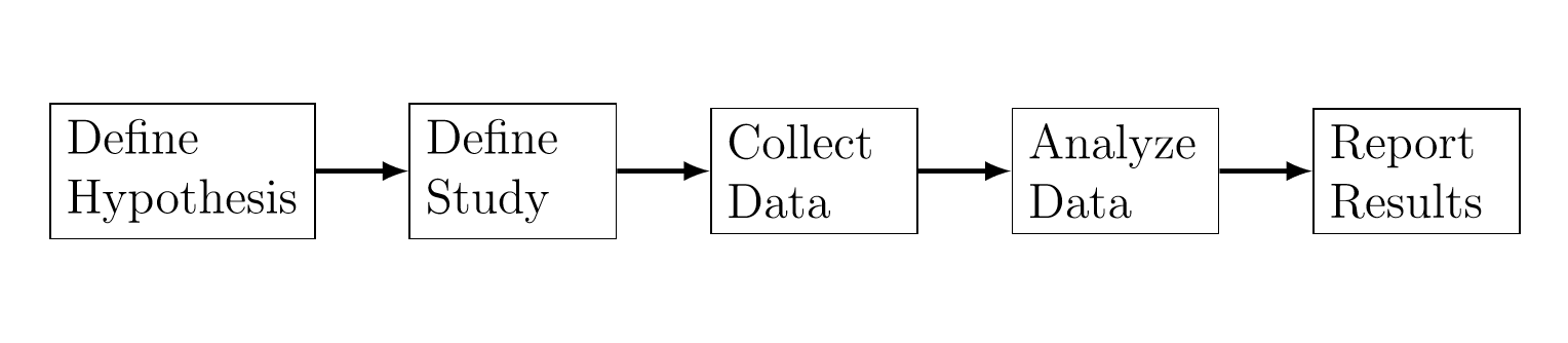
Figure 13.1: The Process of a Typical Study in Behavioral and Social Sciences
Shmueli (2010) described a general process for statistical modeling, which is shown in Figure 13.2. Depending on the goal of the analysis, the steps differ in terms of the choice of methods, criteria, data, and information.
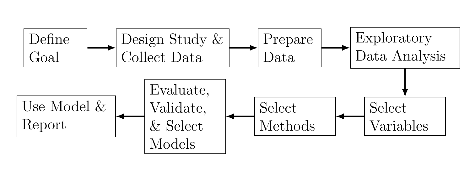
Figure 13.2: The Process of Statistical Modeling
13.2.2 Exploratory versus Confirmatory
There are two phases of data analysis (Good 1983): exploratory data analysisApproach to analyzing data sets to summarize their main characteristics, using visual methods, descriptive statistics, clustering, dimension reduction (EDA) and confirmatory data analysisProcess used to challenge assumptions about the data through hypothesis tests, significance testing, model estimation, prediction, confidence intervals, and inference (CDA). Table 13.1 summarizes some differences between EDA and CDA. EDA is usually applied to observational data with the goal of looking for patterns and formulating hypotheses. In contrast, CDA is often applied to experimental data (i.e., data obtained by means of a formal design of experiments) with the goal of quantifying the extent to which discrepancies between the model and the data could be expected to occur by chance. Gelman (2004).
Table 13.1. Comparison of Exploratory Data Analysis and Confirmatory Data Analysis
\[ \small{ \begin{array}{lll} \hline & \textbf{EDA} & \textbf{CDA} \\\hline \text{Data} & \text{Observational data} & \text{Experimental data}\\[3mm] \text{Goal} & \text{Pattern recognition,} & \text{Hypothesis testing,} \\ & \text{formulate hypotheses} & \text{estimation, prediction} \\[3mm] \text{Techniques} & \text{Descriptive statistics,} & \text{Traditional statistical tools of} \\ & \text{visualization, clustering} & \text{inference, significance, and}\\ & & \text{confidence} \\ \hline \end{array} } \]
Techniques for EDA include descriptive statistics (e.g., mean, median, standard deviation, quantiles), distributions, histograms, correlation analysis, dimension reduction, and cluster analysis. Techniques for CDA include the traditional statistical tools of inference, significance, and confidence.
13.2.3 Supervised versus Unsupervised
Methods for data analysis can be divided into two types (Abbott 2014; Igual and Segu 2017): supervised learning methods and unsupervised learning methods. Supervised learning methodsModel that predicts a response target variable using explanatory predictors as input work with labeled data, which include a target variable. Mathematically, supervised learning methods try to approximate the following function: \[ Y = f(X_1, X_2, \ldots, X_p), \] where \(Y\) is a target variable and \(X_1\), \(X_2\), \(\ldots\), \(X_p\) are explanatory variables. Table 13.2 gives a list of common names for different types of variables (Frees 2009). When the target variable is a categorical variable, supervised learning methods are called classification methodsSupervised learning method where the response is a categorical variable. When the target variable is continuous, supervised learning methods are called regression methodsSupervised learning method where the response is a continuous variable.
Table 13.2. Common Names of Different Variables
\[ \small{ \begin{array}{ll} \hline \textbf{Target Variable} & \textbf{Explanatory Variable}\\\hline \text{Dependent variable} & \text{Independent variable}\\ \text{Response} & \text{Treatment} \\ \text{Output} & \text{Input} \\ \text{Endogenous variable} & \text{Exogenous variable} \\ \text{Predicted variable} & \text{Predictor variable} \\ \text{Regressand} & \text{Regressor} \\ \hline \end{array} } \]
Unsupervised learning methodsModels that work with explanatory variables only to describe patterns or groupings work with unlabeled data, which include explanatory variables only. In other words, unsupervised learning methods do not use target variables. As a result, unsupervised learning methods are also called descriptive modeling methods.
13.2.4 Parametric versus Nonparametric
Methods for data analysis can be parametric or nonparametric (Abbott 2014). Parametric methods assume that the data follow a certain distribution. Nonparametric methods, introduced in Section 4.1, do not assume distributions for the data and therefore are called distribution-free methods.
Parametric methods have the advantage that if the distribution of the data is known, properties of the data and properties of the method (e.g., errors, convergence, coefficients) can be derived. A disadvantage of parametric methods is that analysts need to spend considerable time on figuring out the distribution. For example, analysts may try different transformation methods to transform the data so that it follows a certain distribution.
Because nonparametric methods make fewer assumptions, nonparametric methods have the advantage that they are more flexible, more robustStatistics which are more unaffected by outliers or small departures from model assumptions, and more applicable to non-quantitative data. However, a drawback of nonparametric methods is that it is more difficult to extrapolate findings outside of the observed domain of the data, a key consideration in predictive modeling.
13.2.5 Explanation versus Prediction
There are two goals in data analysis (Breiman 2001; Shmueli 2010): explanation and prediction. In some scientific areas such as economics, psychology, and environmental science, the focus of data analysis is to explain the causal relationships between the input variables and the response variable. In other scientific areas such as natural language processing and bioinformatics, the focus of data analysis is to predict what the responses are going to be given the input variables.
Shmueli (2010) discussed in detail the distinction between explanatory modeling and predictive modeling. Explanatory modeling is commonly used for theory building and testing. However, predictive modeling is rarely used in many scientific fields as a tool for developing theory.
Explanatory modelingProcess where the modeling goal is to identify variables with meaningful and statistically significant relationships and test hypotheses is typically done as follows:
- State the prevailing theory.
- State causal hypotheses, which are given in terms of theoretical constructs rather than measurable variables. A causal diagram is usually included to illustrate the hypothesized causal relationship between the theoretical constructs.
- Operationalize constructs. In this step, previous literature and theoretical justification are used to build a bridge between theoretical constructs and observable measurements.
- Collect data and build models alongside the statistical hypotheses, which are operationalized from the research hypotheses.
- Reach research conclusions and recommend policy. The statistical conclusions are converted into research conclusions or policy recommendations.
Shmueli (2010) defined predictive modelingProcess where the modeling goal is to predict new observations as the process of applying a statistical model or data mining algorithm to data for the purpose of predicting new or future observations. Predictions include point predictions, interval predictions, regions, distributions, and rankings of new observations. A predictive model can be any method that produces predictions.
13.2.6 Data Modeling versus Algorithmic Modeling
Breiman (2001) discussed two cultures for the use of statistical modeling to reach conclusions from data: the data modeling culture and the algorithmic modeling culture. In the data modeling culture, data are assumed to be generated by a given stochastic data model. In the algorithmic modeling culture, the data mechanism is treated as unknown and algorithmic models are used.
Data modelingAssumes data generated comes from a stochastic data model allows statisticians to analyze data and acquire information about the data mechanisms. However, Breiman (2001) argued that the focus on data modeling in the statistical community has led to some side effects such as:
- It produced irrelevant theory and questionable scientific conclusions.
- It kept statisticians from using algorithmic models that might be more suitable.
- It restricted the ability of statisticians to deal with a wide range of problems.
Algorithmic modelingAssumes data generated comes from unknown algorithmic models was used by industrial statisticians long time ago. Sadly, the development of algorithmic methods was taken up by a community outside statistics (Breiman 2001). The goal of algorithmic modeling is predictive accuracyQuantitative measure of how well the explanatory variables predict the response outcome. For some complex prediction problems, data models are not suitable. These prediction problems include speech recognition, image recognition, handwriting recognition, nonlinear time series prediction, and financial market prediction. The theory in algorithmic modeling focuses on the properties of algorithms, such as convergence and predictive accuracy.
13.2.7 Big Data Analysis
Unlike traditional data analysis, big data analysis employs additional methods and tools that can extract information rapidly from massive data. In particular, big data analysis uses the following processing methods (Chen et al. 2014):
- A bloom filter is a space-efficient probabilistic data structure that is used to determine whether an element belongs to a set. It has the advantages of high space efficiency and high query speed. A drawback of using bloom filter is that there is a certain misrecognition rate.
- Hashing is a method that transforms data into fixed-length numerical values through a hash function. It has the advantages of rapid reading and writing. However, sound hash functions are difficult to find.
- Indexing refers to a process of partitioning data in order to speed up reading. Hashing is a special case of indexing.
- A trie, also called digital tree, is a method to improve query efficiency by using common prefixes of character strings to reduce comparisons among character strings.
- Parallel computing uses multiple computing resources to complete a computation task. Parallel computing tools include Message Passing Interface (MPI), MapReduce, and Dryad.
Big data analysis can be conducted in the following levels (Chen et al. 2014): memory-level, business intelligence (BI) level, and massive level. Memory-level analysis is conducted when data can be loaded to the memory of a cluster of computers. Current hardware can handle hundreds of gigabytes (GB) of data in memory. BI level analysis can be conducted when data surpass the memory level. It is common for BI level analysis products to support data over terabytes (TB). Massive level analysis is conducted when data surpass the capabilities of products for BI level analysis. Usually Hadoop and MapReduce are used in massive level analysis.
13.2.8 Reproducible Analysis
As mentioned in Section 13.2.1, a typical data analysis workflow includes collecting data, analyzing data, and reporting results. The data collected are saved in a database or files. Data are then analyzed by one or more scriptsA program or sequence of instructions that is executed by another program, which may save some intermediate results or always work on the raw data. Finally a report is produced to describe the results, which include relevant plots, tables, and summaries of data. The workflow may be subject to the following potential issues (Mailund 2017, Chapter 2):
- Data are separated from the analysis scripts.
- The documentation of the analysis is separated from the analysis itself.
If the analysis is done on the raw data with a single script, then the first issue is not a major problem. If the analysis consists of multiple scripts and a script saves intermediate results that are read by the next script, then the scripts describe a workflow of data analysis. To reproduce an analysis, the scripts have to be executed in the right order. The workflow may cause major problems if the order of the scripts is not documented or the documentation is not updated or lost. One way to address the first issue is to write the scripts so that any part of the workflow can be run automatically at any time.
If the documentation of the analysis is synchronized with the analysis, then the second issue is not a major problem. However, the documentation may become useless if the scripts are changed but the documentation is not updated.
Literate programmingCoding practice where documentation and code are written together is an approach to address the two issues mentioned above, where the documentation of a program and the code of the program are written together. To do literate programming in R, one way is to use R Markdown and the knitr package.
13.2.9 Ethical Issues
Analysts may face ethical issues and dilemmas during the data analysis process. In some fields, ethical issues and dilemmas include participant consent, benefits, risk, confidentiality, and data ownershipGovernance process that details legal ownership of enterprise-wide data and outlines who has ability to create, edit, modify, share and restrict access to the data (Miles, Hberman, and Sdana 2014). For data analysis in actuarial science and insurance in particular, we face the following ethical matters and issues (Miles, Hberman, and Sdana 2014):
- Worthiness of the project. Is the project worth doing? Will the project contribute in some significant way to a domain broader than my career? If a project is only opportunistic and does not have a larger significance, then it might be pursued with less care. The result may look good but not be right.
- Competence. Do I or the whole team have the expertise to carry out the project? Incompetence may lead to weakness in the analytics such as collecting large amounts of data poorly and drawing superficial conclusions.
- Benefits, costs, and reciprocity. Will each stakeholder gain from the project? Are the benefits and costs equitable? A project will likely to fail if the benefit and the cost for a stakeholder do not match.
- Privacy and confidentiality. How do we make sure that the information is kept confidentially? How do we verify where are raw data and analysis results stored? How will we have access to them? These questions should be addressed and documented in explicit confidentiality agreements.
Show Quiz Solution
13.3 Data Analysis Techniques
Techniques for data analysis are drawn from different but overlapping fields such as statistics, machine learning, pattern recognition, and data mining. Statistics is a field that addresses reliable ways of gathering data and making inferences, Bandyopadhyay and Forster (2011), Bluman (2012). The term machine learningStudy of algorithms and statistical models that perform a specific task without using explicit instructions, relying on patterns and inference was coined by Samuel in 1959 (Samuel 1959). Originally, machine learning referred to the field of study where computers have the ability to learn without being explicitly programmed. Nowadays, machine learning has evolved to the broad field of study where computational methods use experience (i.e., the past information available for analysis) to improve performance or to make accurate predictions (Bishop 2007; Clarke, Fokoue, and Zhang 2009; Mohri, Rostamizadeh, and Talwalkar 2012; Kubat 2017). There are four types of machine learning algorithms (see Table 13.3) depending on the type of data and the type of the learning tasks.
Table 13.3. Types of Machine Learning Algorithms
\[ \small{ \begin{array}{rll} \hline & \textbf{Supervised} & \textbf{Unsupervised} \\\hline \textbf{Discrete Data} & \text{Classification} & \text{Clustering} \\ \textbf{Continuous Data} & \text{Regression} & \text{Dimension reduction} \\ \hline \end{array} } \]
Originating in engineering, pattern recognitionAutomated recognition of patterns and regularities in data is a field that is closely related to machine learning, which grew out of computer science. In fact, pattern recognition and machine learning can be considered to be two facets of the same field (Bishop 2007). Data miningProcess of collecting, cleaning, processing, analyzing, and discovering patterns and useful insights from large data sets is a field that concerns collecting, cleaning, processing, analyzing, and gaining useful insights from data (Aggarwal 2015).
13.3.1 Exploratory Techniques
Exploratory data analysis techniques include descriptive statistics as well as many unsupervised learning techniques such as data clustering and principal component analysis.
13.3.1.1 Descriptive Statistics
In one sense (as a “mass noun”), “descriptive statistics” is an area of statistics that concerns the collection, organization, summarization, and presentation of data (Bluman 2012). In another sense (as a “count noun”), “descriptive statistics” are summary statistics that quantitatively describe or summarize data.
Table 13.4. Commonly Used Descriptive Statistics
\[ \small{ \begin{array}{ll} \hline & \textbf{Descriptive Statistics} \\\hline \text{Measures of central tendency} & \text{Mean, median, mode, midrange}\\ \text{Measures of variation} & \text{Range, variance, standard deviation} \\ \text{Measures of position} & \text{Quantile} \\ \hline \end{array} } \]
Table 13.4 lists some commonly used descriptive statistics. In R, we can use the function summary to calculate some of the descriptive statistics. For numeric data, we can visualize the descriptive statistics using a boxplot.
In addition to these quantitative descriptive statistics, we can also qualitatively describe shapes of the distributions (Bluman 2012). For example, we can say that a distribution is positively skewed, symmetric, or negatively skewed. To visualize the distribution of a variable, we can draw a histogram.
13.3.1.2 Principal Component Analysis
Principal component analysisDimension reduction technique that uses orthogonal transformations to convert a set of possibly correlated variables into a set of linearly uncorrelated variables (PCA) is a statistical procedure that transforms a dataset described by possibly correlated variables into a dataset described by linearly uncorrelated variables, which are called principal components and are ordered according to their variances. PCA is a technique for dimension reduction. If the original variables are highly correlated, then the first few principal components can account for most of the variation of the original data.
The principal components of the variables are related to the eigenvalues and eigenvectors of the covariance matrix of the variables. For \(i=1,2,\ldots,d\), let \((\lambda_i, \textbf{e}_i)\) be the \(i\)th eigenvalue-eigenvector pair of the covariance matrix \({\Sigma}\) of \(d\) variables \(X_1,X_2,\ldots,X_d\) such that \(\lambda_1\ge \lambda_2\ge \ldots\ge \lambda_d\ge 0\) and the eigenvectors are normalized. Then the \(i\)th principal component is given by
\[ Z_{i} = \textbf{e}_i' \textbf{X} =\sum_{j=1}^d e_{ij} X_j, \]
where \(\textbf{X}=(X_1,X_2,\ldots,X_d)'\). It can be shown that \(\mathrm{Var~}{(Z_i)} = \lambda_i\). As a result, the proportion of variance explained by the \(i\)th principal component is calculated as
\[ \frac{\mathrm{Var~}{(Z_i)}}{ \sum_{j=1}^{d} \mathrm{Var~}{(Z_j)}} = \frac{\lambda_i}{\lambda_1+\lambda_2+\cdots+\lambda_d}. \]
For more information about PCA, readers are referred to Mirkin (2011).
13.3.1.3 Cluster Analysis
Cluster analysisUnsupervised learning method that aims to splot data into homogenous groups using a similarity measure (aka data clustering) refers to the process of dividing a dataset into homogeneous groups or clusters such that points in the same cluster are similar and points from different clusters are quite distinct (Gan, Ma, and Wu 2007; Gan 2011). Data clustering is one of the most popular tools for exploratory data analysis and has found its applications in many scientific areas.
During the past several decades, many clustering algorithms have been proposed. Among these clustering algorithms, the \(k\)-means algorithm is perhaps the most well-known algorithm due to its simplicity. To describe the k-means algorithmType of clustering that aims to partition data into k mutually exclusive clusters by assigning observations to the cluster with the nearest centroid, let \(X=\{\textbf{x}_1,\textbf{x}_2,\ldots,\textbf{x}_n\}\) be a dataset containing \(n\) points, each of which is described by \(d\) numerical features. Given a desired number of clusters \(k\), the \(k\)-means algorithm aims at minimizing the following objective function:
\[ P(U,Z) = \sum_{l=1}^k\sum_{i=1}^n u_{il} \Vert \textbf{x}_i-\textbf{z}_l\Vert^2, \]
where \(U=(u_{il})_{n\times k}\) is an \(n\times k\) partition matrix, \(Z=\{\textbf{z}_1,\textbf{z}_2,\ldots,\textbf{z}_k\}\) is a set of cluster centers, and \(\Vert\cdot\Vert\) is the \(L^2\) norm or Euclidean distance. The partition matrix \(U\) satisfies the following conditions:
\[ u_{il}\in \{0,1\},\quad i=1,2,\ldots,n,\:l=1,2,\ldots,k, \]
\[ \sum_{l=1}^k u_{il}=1,\quad i=1,2,\ldots,n. \]
The \(k\)-means algorithm employs an iterative procedure to minimize the objective function. It repeatedly updates the partition matrix \(U\) and the cluster centers \(Z\) alternately until some stop criterion is met. For more information about \(k\)-means, readers are referred to Gan, Ma, and Wu (2007) and Mirkin (2011).
13.3.2 Confirmatory Techniques
Confirmatory data analysis techniques include the traditional statistical tools of inference, significance, and confidence.
13.3.2.1 Linear Models
Linear models, also called linear regression modelsSupervised model that uses a linear function to approximate the relationship between the target and explanatory variables, aim at using a linear function to approximate the relationship between the dependent variable and independent variables. A linear regression model is called a simple linear regression model if there is only one independent variable. When more than one independent variable is involved, a linear regression model is called a multiple linear regression model.
Let \(X\) and \(Y\) denote the independent and the dependent variables, respectively. For \(i=1,2,\ldots,n\), let \((x_i, y_i)\) be the observed values of \((X,Y)\) in the \(i\)th case. Then the simple linear regression model is specified as follows (Frees 2009):
\[ y_i = \beta_0 + \beta_1 x_i + \epsilon_i,\quad i=1,2,\ldots,n, \]
where \(\beta_0\) and \(\beta_1\) are parameters and \(\epsilon_i\) is a random variable representing the error for the \(i\)th case.
When there are multiple independent variables, the following multiple linear regression model is used:
\[ y_i = \beta_0 + \beta_1 x_{i1} + \cdots + \beta_k x_{ik} + \epsilon_i, \]
where \(\beta_0\), \(\beta_1\), \(\ldots\), \(\beta_k\) are unknown parameters to be estimated.
Linear regression models usually make the following assumptions:
- \(x_{i1},x_{i2},\ldots,x_{ik}\) are nonstochastic variables.
- \(\mathrm{Var~}(y_i)=\sigma^2\), where \(\mathrm{Var~}(y_i)\) denotes the variance of \(y_i\).
- \(y_1,y_2,\ldots,y_n\) are independent random variables.
For the purpose of obtaining tests and confidence statements with small samples, the following strong normality assumption is also made:
- \(\epsilon_1,\epsilon_2,\ldots,\epsilon_n\) are normally distributed.
13.3.2.2 Generalized Linear Models
The generalized linear modelSupervised model that generalizes linear regression by allowing the linear component to be related to the response variable via a link function and by allowing the variance of each measurement to be a function of its predicted value (GLM) consists of a wide family of regression models that include linear regression models as a special case. In a GLM, the mean of the response (i.e., the dependent variable) is assumed to be a function of linear combinations of the explanatory variables, i.e.,
\[ \mu_i = \mathrm{E}~[y_i], \]
\[ \eta_i = \textbf{x}_i'\boldsymbol{\beta} = g(\mu_i), \]
where \(\textbf{x}_i=(1,x_{i1}, x_{i2}, \ldots, x_{ik})'\) is a vector of regressor values, \(\mu_i\) is the mean response for the \(i\)th case, and \(\eta_i\) is a systematic componentThe linear combination of explanatory variables component in a glm of the GLMGeneralized linear model. The function \(g(\cdot)\) is known and is called the link functionFunction that relates between the linear predictor component to the mean of the target variable. The mean response can vary by observations by allowing some parameters to change. However, the regression parameters \(\boldsymbol{\beta}\) are assumed to be the same among different observations.
GLMs make the following assumptions:
- \(x_{i1},x_{i2},\ldots,x_{in}\) are nonstochastic variables.
- \(y_1,y_2,\ldots,y_n\) are independent.
- The dependent variable is assumed to follow a distribution from the linear exponential family.
- The variance of the dependent variable is not assumed to be constant but is a function of the mean, i.e.,
\[ \mathrm{Var~}{(y_i)} = \phi \nu(\mu_i), \]
where \(\phi\) denotes the dispersion parameter and \(\nu(\cdot)\) is a function.
As we can see from the above specification, the GLM provides a unifying framework to handle different types of dependent variables, including discrete and continuous variables. For more information about GLMs, readers are referred to De Jong and Heller (2008) and Frees (2009).
13.3.2.3 Tree-based Models
Decision treesModeling technique that uses a tree-like model of decisions to divide the sample space into non-overlapping regions to make predictions, also known as tree-based models, involve dividing the predictor space (i.e., the space formed by independent variables) into a number of simple regions and using the mean or the mode of the region for prediction (Breiman et al. 1984). There are two types of tree-based models: classification trees and regression trees. When the dependent variable is categorical, the resulting tree models are called classification trees. When the dependent variable is continuous, the resulting tree models are called regression trees.
The process of building classification trees is similar to that of building regression trees. Here we only briefly describe how to build a regression tree. To do that, the predictor space is divided into non-overlapping regions such that the following objective function
\[ f(R_1,R_2,\ldots,R_J) = \sum_{j=1}^J \sum_{i=1}^n I_{R_j}(\textbf{x}_i)(y_i - \mu_j)^2 \]
is minimized, where \(I\) is an indicator function, \(R_j\) denotes the set of indices of the observations that belong to the \(j\)th box, \(\mu_j\) is the mean response of the observations in the \(j\)th box, \(\textbf{x}_i\) is the vector of predictor values for the \(i\)th observation, and \(y_i\) is the response value for the \(i\)th observation.
In terms of predictive accuracy, decision trees generally do not perform to the level of other regression and classification models. However, tree-based models may outperform linear models when the relationship between the response and the predictors is nonlinear. For more information about decision trees, readers are referred to Breiman et al. (1984) and Mitchell (1997).
Show Quiz Solution
13.4 Some R Functions
R is an open-source software for statistical computing and graphics. The R software can be downloaded from the R project website at https://www.r-project.org/. In this section, we give some R function for data analysis, especially the data analysis tasks mentioned in previous sections.
Table 13.5. Some R Functions for Data Analysis
\[ \small{ \begin{array}{lll} \hline \text{Data Analysis Task} & \text{R Package} & \text{R Function} \\\hline \text{Descriptive Statistics} & \texttt{base} & \texttt{summary}\\ \text{Principal Component Analysis} & \texttt{stats} & \texttt{prcomp} \\ \text{Data Clustering} & \texttt{stats} & \texttt{kmeans}, \texttt{hclust} \\ \text{Fitting Distributions} & \texttt{MASS} & \texttt{fitdistr} \\ \text{Linear Regression Models} & \texttt{stats} & \texttt{lm} \\ \text{Generalized Linear Models} & \texttt{stats} & \texttt{glm} \\ \text{Regression Trees} & \texttt{rpart} & \texttt{rpart} \\ \text{Survival Analysis} & \texttt{survival} & \texttt{survfit} \\ \hline \end{array} } \]
Table 13.5 lists a few R functions for different data analysis tasks. Readers can go to the R documentation to learn how to use these functions. There are also other R packages that do similar things. However, the functions listed in this table provide good starting points for readers to conduct data analysis in R. For analyzing large datasets in R in an efficient way, readers are referred to Daroczi (2015).
13.5 Summary
In this chapter, we give a high-level overview of data analysis by introducing data types, data structures, data storages, data sources, data analysis processes, and data analysis techniques. In particular, we present various aspects of data analysis. In addition, we provide several websites where readers can obtain real-world datasets to hone their data analysis skills. We also list some R packages and functions that can be used to perform various data analysis tasks.
13.6 Further Resources and Contributors
Contributor
- Guojun Gan, University of Connecticut, is the principal author of the initial version of this chapter. Email: guojun.gan@uconn.edu for chapter comments and suggested improvements.
- Chapter reviewers include: Runhuan Feng, Himchan Jeong, Lei Hua, Min Ji, and Toby White.
Bibliography
Abbott, Dean. 2014. Applied Predictive Analytics: Principles and Techniques for the Professional Data Analyst. Hoboken, NJ: Wiley.
Abdullah, Mohammad F., and Kamsuriah Ahmad. 2013. “The Mapping Process of Unstructured Data to Structured Data.” In 2013 International Conference on Research and Innovation in Information Systems (Icriis), 151–55.
Aggarwal, Charu C. 2015. Data Mining: The Textbook. New York, NY: Springer.
Albers, Michael J. 2017. Introduction to Quantitative Data Analysis in the Behavioral and Social Sciences. Hoboken, NJ: John Wiley & Sons, Inc.
Bandyopadhyay, Prasanta S., and Malcolm R. Forster, eds. 2011. Philosophy of Statistics. Handbook of the Philosophy of Science 7. North Holland.
Bishop, Christopher M. 2007. Pattern Recognition and Machine Learning. New York, NY: Springer.
Bluman, Allan. 2012. Elementary Statistics: A Step by Step Approach. New York, NY: McGraw-Hill.
Breiman, Leo. 2001. “Statistical Modeling: The Two Cultures.” Statistical Science 16 (3): 199–231.
Breiman, Leo, Jerome Friedman, Charles J. Stone, and R. A. Olshen. 1984. Classification and Regression Trees. Raton Boca, FL: Chapman; Hall/CRC.
Buttrey, Samuel E., and Lyn R. Whitaker. 2017. A Data Scientist’s Guide to Acquiring, Cleaning, and Managing Data in R. Hoboken, NJ: Wiley.
Chen, Min, Shiwen Mao, Yin Zhang, and Victor CM Leung. 2014. Big Data: Related Technologies, Challenges and Future Prospects. New York, NY: Springer.
Clarke, Bertrand, Ernest Fokoue, and Hao Helen Zhang. 2009. Principles and Theory for Data Mining and Machine Learning. New York, NY: Springer-Verlag.
Daroczi, Gergely. 2015. Mastering Data Analysis with R. Birmingham, UK: Packt Publishing.
De Jong, Piet, and Gillian Z. Heller. 2008. Generalized Linear Models for Insurance Data. Cambridge University Press, Cambridge.
Forte, Rui Miguel. 2015. Mastering Predictive Analytics with R. Birmingham, UK: Packt Publishing.
Frees, Edward W. 2009. Regression Modeling with Actuarial and Financial Applications. Cambridge University Press.
Gan, Guojun. 2011. Data Clustering in C++: An Object-Oriented Approach. Data Mining and Knowledge Discovery Series. Boca Raton, FL, USA: Chapman & Hall/CRC Press. https://doi.org/10.1201/b10814.
Gan, Guojun, Chaoqun Ma, and Jianhong Wu. 2007. Data Clustering: Theory, Algorithms, and Applications. Philadelphia, PA: SIAM Press. https://doi.org/10.1137/1.9780898718348.
Gelman, Andrew. 2004. “Exploratory Data Analysis for Complex Models.” Journal of Computational and Graphical Statistics 13 (4): 755–79.
Good, I. J. 1983. “The Philosophy of Exploratory Data Analysis.” Philosophy of Science 50 (2): 283–95.
Hashem, Ibrahim Abaker Targio, Ibrar Yaqoob, Nor Badrul Anuar, Salimah Mokhtar, Abdullah Gani, and Samee Ullah Khan. 2015. “The Rise of ‘Big Data’ on Cloud Computing: Review and Open Research Issues.” Information Systems 47: 98–115.
Hox, Joop J., and Hennie R. Boeije. 2005. “Data Collection, Primary Versus Secondary.” In Encyclopedia of Social Measurement, 593–99. Elsevier.
Igual, Laura, and Santi Segu. 2017. Introduction to Data Science. A Python Approach to Concepts, Techniques and Applications. New York, NY: Springer.
Inmon, W. H., and Dan Linstedt. 2014. Data Architecture: A Primer for the Data Scientist: Big Data, Data Warehouse and Data Vault. Cambridge, MA: Morgan Kaufmann.
Janert, Philipp K. 2010. Data Analysis with Open Source Tools. Sebastopol, CA: O’Reilly Media.
Judd, Charles M., Gary H. McClelland, and Carey S. Ryan. 2017. Data Analysis. A Model Comparison Approach to Regression, ANOVA and Beyond. 3rd ed. New York, NY: Routledge.
Kubat, Miroslav. 2017. An Introduction to Machine Learning. 2nd ed. New York, NY: Springer.
Mailund, Thomas. 2017. Beginning Data Science in R: Data Analysis, Visualization, and Modelling for the Data Scientist. Apress.
Miles, Matthew, Michael Hberman, and Johnny Sdana. 2014. Qualitative Data Analysis: A Methods Sourcebook. 3rd ed. Thousand Oaks, CA: Sage.
Mirkin, Boris. 2011. Core Concepts in Data Analysis: Summarization, Correlation and Visualization. London, UK: Springer.
Mitchell, Tom M. 1997. Machine Learning. McGraw-Hill.
Mohri, Mehryar, Afshin Rostamizadeh, and Ameet Talwalkar. 2012. Foundations of Machine Learning. Cambridge, MA: MIT Press.
O’Leary, D. E. 2013. “Artificial Intelligence and Big Data.” IEEE Intelligent Systems 28 (2): 96–99.
Olson, Jack E. 2003. Data Quality: The Accuracy Dimension. San Francisco, CA: Morgan Kaufmann.
Pries, Kim H., and Robert Dunnigan. 2015. Big Data Analytics: A Practical Guide for Managers. Boca Raton, FL: CRC Press.
Samuel, A. L. 1959. “Some Studies in Machine Learning Using the Game of Checkers.” IBM Journal of Research and Development 3 (3): 210–29.
Shmueli, Galit. 2010. “To Explain or to Predict?” Statistical Science 25 (3): 289–310.
Tukey, John W. 1962. “The Future of Data Analysis.” The Annals of Mathematical Statistics 33 (1): 1–67.