Chapter 14 Dependence Modeling
Chapter Preview. In practice, there are many types of variables that one encounters. The first step in dependence modeling is identifying the type of variable to help direct you to the appropriate technique. This chapter introduces readers to variable types and techniques for modeling dependence or association of multivariate distributions. Section 14.1 provides an overview of the types of variables. Section 14.2 then elaborates basic measures for modeling the dependence between variables.
Section 14.3 introduces an approach to modeling dependence using copulas which is reinforced with practical illustrations in Section 14.4. The types of copula families and basic properties of copula functions are explained Section 14.5. The chapter concludes by explaining why the study of dependence modeling is important in Section 14.6.
14.1 Variable Types
In this section, you learn how to:
- Classify variables as qualitative or quantitative.
- Describe multivariate variables.
People, firms, and other entities that we want to understand are described in a dataset by numerical characteristics. As these characteristics vary by entity, they are commonly known as variablesA variable is any characteristics, number, or quantity that can be measured or counted.. To manage insurance systems, it will be critical to understand the distribution of each variable and how they are associated with one another. It is common for data sets to have many variables (high dimensionalData set is high dimensional when it has many variables. In many applications, the number of variables may be larger than the sample size.) and so is useful to begin by classifying them into different types. As will be seen, these classifications are not strict; there is overlap among the groups. Nonetheless, the grouping summarized in Table 14.1 and explained in the remainder of this section provides a solid first step in framing a data set.
Table 14.1. Variable Types
\[ {\small \begin{matrix} \begin{array}{l|l} \hline \textbf{Variable Type} & \textbf{Example} \\\hline Qualitative & \\ \text{Binary} & \text{Sex} \\ \text{Categorical (Unordered, Nominal)} & \text{Territory (e.g., state/province) in which an insured resides} \\ \text{Ordered Category (Ordinal)} & \text{Claimant satisfaction (five point scale ranging from 1=dissatisfied} \\ & ~~~ \text{to 5 =satisfied)} \\\hline Quantitative & \\ \text{Continuous} & \text{Policyholder's age, weight, income} \\ \text{Discrete} & \text{Amount of deductible (0, 250, 500, and 1000)} \\ \text{Count} & \text{Number of insurance claims} \\ \text{Combinations of} & \text{Policy losses, mixture of 0's (for no loss)} \\ ~~~ \text{Discrete and Continuous} & ~~~\text{and positive claim amount} \\ \text{Interval Variable} & \text{Driver Age: 16-24 (young), 25-54 (intermediate),} \\ & ~~~\text{55 and over (senior)} \\ \text{Circular Data} & \text{Time of day measures of customer arrival} \\ \hline Multivariate ~ Variable & \\ \text{High Dimensional Data} & \text{Characteristics of a firm purchasing worker's compensation} \\ & ~~~\text{insurance (location of plants, industry, number of employees,} \\ &~~~\text{and so on)} \\ \text{Spatial Data} & \text{Longitude/latitude of the location an insurance hailstorm claim} \\ \text{Missing Data} & \text{Policyholder's age (continuous/interval) and -99 for} \\ &~~~ `\text{not reported,' that is, missing} \\ \text{Censored and Truncated Data} & \text{Amount of insurance claims in excess of a deductible} \\ \text{Aggregate Claims} & \text{Losses recorded for each claim in a motor vehicle policy.} \\ \text{Stochastic Process Realizations} & \text{The time and amount of each occurrence of an insured loss} \\ \hline \end{array} \end{matrix}} \]
In data analysis, it is important to understand what type of variable you are working with. For example, consider a pair of random variables \({\tt (Coverage, Claim)}\) from the LGPIF data introduced in Section 1.3 as displayed in Figure 14.1 below. We would like to know whether the distribution of \({\tt Coverage}\) depends on the distribution of \({\tt Claim}\) or whether they are statistically independent. We would also want to know how the \({\tt Claim}\) distribution depends on the \({\tt EntityType}\) variable. Because the \({\tt EntityType}\) variable belongs to a different class of variables, modeling the dependence between \({\tt Claim}\) and \({\tt Coverage}\) may require a different technique from that of \({\tt Claim}\) and \({\tt EntityType}\).
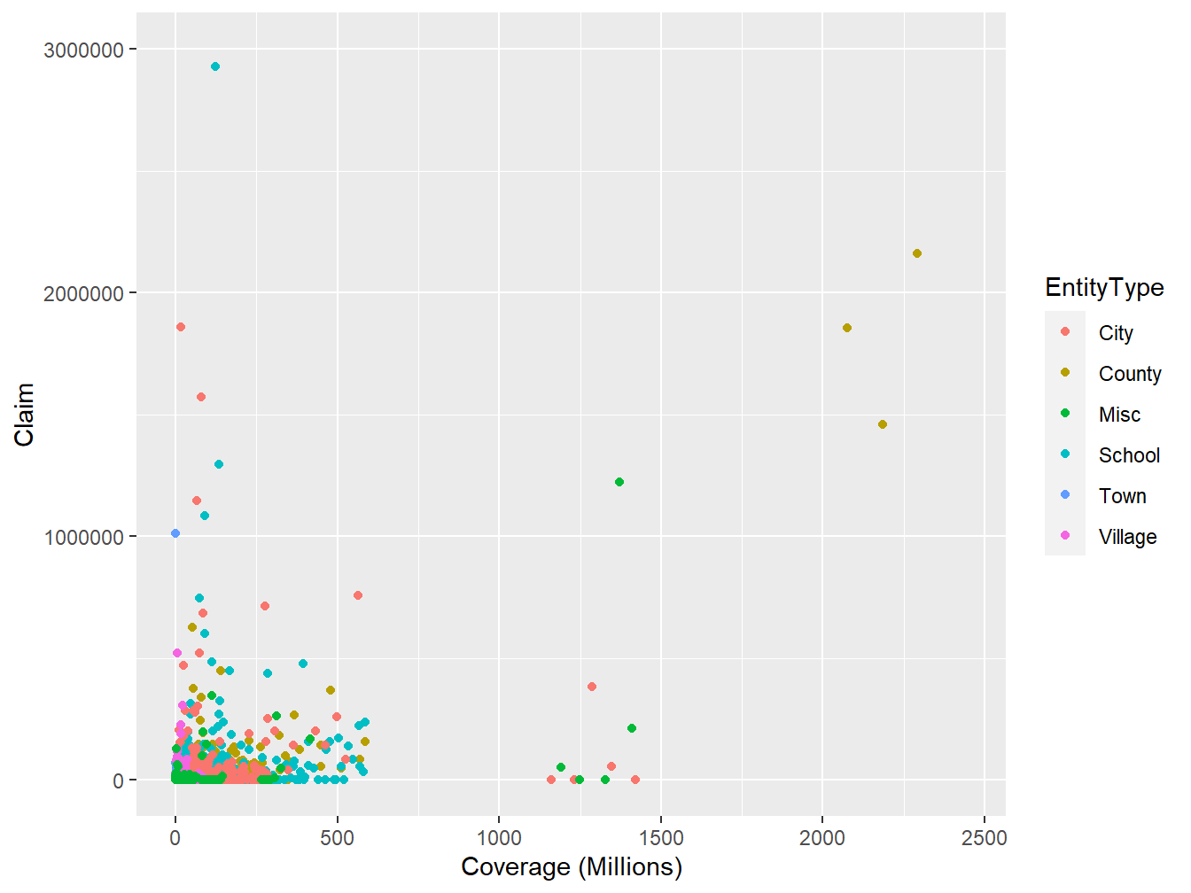
Figure 14.1: Scatter Plot of (Coverage,Claim) from LGPIF Data
14.1.1 Qualitative Variables
In this sub-section, you learn how to:
- Classify qualitative variables as nominal or ordinal
- Describe a binary variable
A qualitativeThis is a type of variable in which the measurement denotes membership in a set of groups, or categories, or categorical variableA variable whose values are qualitative groups and can have no natural ordering (nominal) or an ordering (ordinal) is one for which the measurement denotes membership in a set of groups, or categories. For example, if you were coding in which area of the country an insured resides, you might use 1 for the northern part, 2 for southern, and 3 for everything else. This location variable is an example of a nominal variableThis is a type of qualitative/ categorical variable which has two or more categories without having any kind of natural order., one for which the levels have no natural ordering. Any analysis of nominal variables should not depend on the labeling of the categories. For example, instead of using a 1,2,3 for north, south, other, I should arrive at the same set of summary statistics if I used a 2,1,3 coding instead, interchanging north and south.
In contrast, an ordinal variableThis is a type of qualitative/ categorical variable which has two or more ordered categories. is a type of categorical variable for which an ordering does exist. For example, with a survey to see how satisfied customers are with our claims servicing department, we might use a five point scale that ranges from 1 meaning dissatisfied to a 5 meaning satisfied. Ordinal variables provide a clear ordering of levels of a variable but the amount of separation between levels is unknown.
A binary variableIs a special type of categorical variable where there are only two categories. is a special type of categorical variable where there are only two categories commonly taken to be 0 and 1. For example, we might code a variable in a dataset to be 1 if an insured is female and 0 if male.
14.1.2 Quantitative Variables
In this sub-section, you learn how to:
- Differentiate between continuous and discrete variables
- Use a combination of continuous and discrete variables
- Describe circular data
Unlike a qualitative variable, a quantitative variableA quantitative variable is a type of variable in which numerical level is a realization from some scale so that the distance between any two levels of the scale takes on meaning. is one in which each numerical level is a realization from some scale so that the distance between any two levels of the scale takes on meaning. A continuous variableA continuous variable is a quantitative variable that can take on any value within a finite interval. is one that can take on any value within a finite interval. For example, one could represent a policyholderPerson in actual possession of insurance policy; policy owner.’s age, weight, or income, as continuous variables. In contrast, a discrete variableA discrete variable is quantitative variable that takes on only a finite number of values in any finite interval. is one that takes on only a finite number of values in any finite interval. For example, when examining a policyholder’s choice of deductiblesA deductible is a parameter specified in the contract. Typically, losses below the deductible are paid by the policyholder whereas losses in excess of the deductible are the insurer’s responsibility (subject to policy limits and coninsurance)., it may be that values of 0, 250, 500, and 1000 are the only possible outcomes. Like an ordinal variable, these represent distinct categories that are ordered. Unlike an ordinal variable, the numerical difference between levels takes on economic meaning. A special type of discrete variable is a count variableA count variable is a discrete variable with values on nonnegative integers., one with values on the nonnegative integers. For example, we will be particularly interested in the number of claims arising from a policy during a given period.
Some variables are inherently a combination of discrete and continuous components. For example, when we analyze the insured lossThe amount of damages sustained by an individual or corporation, typically as the result of an insurable event. of a policyholder, we will encounter a discrete outcome at zero, representing no insured loss, and a continuous amount for positive outcomes, representing the amount of the insured loss. Another interesting variation is an interval variableAn ordinal variable with the additional property that the magnitudes of the differences between two values are meaningful, one that gives a range of possible outcomes.
Circular dataIn a circular data, all values around the circle are equally likely. Example, imagine an analog picture of a clock. represent an interesting category typically not analyzed by insurersAn insurance company authorized to write insurance under the laws of any state.. As an example of circular data, suppose that you monitor calls to your customer service center and would like to know when is the peak time of the day for calls to arrive. In this context, one can think about the time of the day as a variable with realizations on a circle, e.g., imagine an analog picture of a clock. For circular data, the distance between observations at 00:15 and 00:45 are just as close as observations 23:45 and 00:15 (the convention HH:MM means hours and minutes).
14.1.3 Multivariate Variables
In this sub-section, you learn how to:
- Differentiate between univariate and multivariate data
- Handle missing variables
Insurance data typically are multivariateMultivariate variable involves taking many measurements on a single entity. in the sense that we can take many measurements on a single entity. For example, when studying losses associated with a firm’s workers’ compensationInsurance that covers an employer’s liability for injuries, disability or death to persons in their employment, without regard to fault, as prescribed by state or federal workers’ compensation laws and other statutes. plan, we might want to know the location of its manufacturing plants, the industry in which it operates, the number of employees, and so forth. The usual strategy for analyzing multivariate data is to begin by examining each variable in isolation of the others. This is known as a univariateUnivariate analysis is the simplest form of analyzing data. “Uni” means “one”, so in other words your data has only one variable. approach.
In contrast, for some variables, it makes little sense to only look at one dimensional aspect. For example, insurers typically organize spatial dataData and information having an implicit or explicit association with a location relative to the earth by longitude and latitude to analyze the location of weather related insurance claims due to hailstorms. Having only a single number, either longitude or latitude, provides little information in understanding geographic location.
Another special case of a multivariate variable, less obvious, involves coding for missing dataMissing data occur when no data value is stored for a variable in an observation. Missing data can occur because of nonresponse: no information is provided for one or more items or for a whole unit or subject.. Historically, some statistical packages used a -99 to report when a variable, such as policyholder’s age, was not available or not reported. This led to many unsuspecting analysts providing strange statistics when summarizing a set of data. When data are missing, it is better to think about the variable as having two dimensions, one to indicate whether or not the variable is reported and the second providing the age (if reported). In the same way, insurance data are commonly censoredCensored data have unknown values beyond a bound on either end of the number line or both. Here, the data is observed but the values (measurements) are not known completely. and truncatedTruncation occurs when values beyond a boundary are either excluded when gathered or excluded when analyzed. An object can be detected only if its value is greater than some number.. We refer you to Section 4.3 for more on censored and truncated data. Aggregate claimsThe sum of all claims observed in a period of time, described in Chapter 5, can also be coded as another special type of multivariate variable.
Perhaps the most complicated type of multivariate variable is a realization of a stochastic processStochastic process is defined as a collection of random variables that is indexed by some mathematical set, meaning that each random variable of the stochastic process is uniquely associated with an element in the set.. You will recall that a stochastic process is little more than a collection of random variables. For example, in insurance, we might think about the times that claims arrive to an insurance company in a one-year time horizon. This is a high dimensional variable that theoretically is infinite dimensional. Special techniques are required to understand realizations of stochastic processes that will not be addressed here.
Show Quiz Solution
14.2 Classic Measures of Scalar Associations
In this section, you learn how to:
- Estimate correlation using the Pearson method
- Use rank based measures like Spearman, Kendall to estimate correlation
- Measure dependence using the odds ratio, Pearson chi-square, and likelihood ratio test statistics
- Use normal-based correlations to quantify associations involving ordinal variables
14.2.1 Association Measures for Quantitative Variables
For this section, consider a pair of random variables \((X,Y)\) having joint distribution function \(F(\cdot)\) and a random sample \((X_i,Y_i), i=1, \ldots, n\). For the continuous case, suppose that \(F(\cdot)\) has absolutely continuous marginals with marginal density functions.
14.2.1.1 Pearson Correlation
Define the sample covariance function \(\widehat{Cov}(X,Y) = \frac{1}{n} \sum_{i=1}^n (X_i - \bar{X})(Y_i - \bar{Y})\), where \(\bar{X}\) and \(\bar{Y}\) are the sample means of \(X\) and \(Y\), respectively. Then, the product-moment (Pearson) correlationPearson correlation, a measure of the linear correlation between two variables can be written as
\[ r = \frac{\widehat{Cov}(X,Y)}{\sqrt{\widehat{Cov}(X,X)\widehat{Cov}(Y,Y)}} = \frac{\widehat{Cov}(X,Y)}{\sqrt{\widehat{Var}(X)}\sqrt{\widehat{Var}(Y)}}. \]
The correlation statistic \(r\) is widely used to capture linear association between random variables. It is a (nonparametric) estimator of the correlation parameter \(\rho\), defined to be the covariance divided by the product of standard deviations.
This statistic has several important features. Unlike regression estimators, it is symmetric between random variables, so the correlation between \(X\) and \(Y\) equals the correlation between \(Y\) and \(X\). It is unchanged by linear transformations of random variables (up to sign changes) so that we can multiply random variables or add constants as is helpful for interpretation. The range of the statistic is \([-1,1]\) which does not depend on the distribution of either \(X\) or \(Y\).
Further, in the case of independence, the correlation coefficient \(r\) is 0. However, it is well known that zero correlation does not in general imply independence, one exception is the case of normally distributed random variables. The correlation statistic \(r\) is also a (maximum likelihood) estimator of the association parameter for the bivariate normal distribution. So, for normally distributed data, the correlation statistic \(r\) can be used to assess independence. For additional interpretations of this well-known statistic, readers will enjoy Lee Rodgers and Nicewander (1998).
You can obtain the Pearson correlationA measure of the linear correlation between two variables statistic \(r\) using the cor() function in R and selecting the pearson method. This is demonstrated below by using the \({\tt Coverage}\) rating variable in millions of dollars and \({\tt Claim}\) amount variable in dollars from the LGPIF data introduced in chapter 1.
R Code for Pearson Correlation Statistic
From the R output above, \(r=0.31\), which indicates a positive association between \({\tt Claim}\) and \({\tt Coverage}\). This means that as the coverage amount of a policy increases we expect claims to increase.
14.2.2 Rank Based Measures
14.2.2.1 Spearman’s Rho
The Pearson correlation coefficient does have the drawback that it is not invariant to nonlinear transforms of the data. For example, the correlation between \(X\) and \(\log Y\) can be quite different from the correlation between \(X\) and \(Y\). As we see from the R code for the Pearson correlation statistic above, the correlation statistic \(r\) between the \({\tt Coverage}\) rating variable in logarithmic millions of dollars and the \({\tt Claim}\) amounts variable in dollars is \(0.1\) as compared to \(0.31\) when we calculate the correlation between the \({\tt Coverage}\) rating variable in millions of dollars and the \({\tt Claim}\) amounts variable in dollars. This limitation is one reason for considering alternative statistics.
Alternative measures of correlation are based on ranks of the data. Let \(R(X_j)\) denote the rank of \(X_j\) from the sample \(X_1, \ldots, X_n\) and similarly for \(R(Y_j)\). Let \(R(X) = \left(R(X_1), \ldots, R(X_n)\right)'\) denote the vector of ranks, and similarly for \(R(Y)\). For example, if \(n=3\) and \(X=(24, 13, 109)\), then \(R(X)=(2,1,3)\). A comprehensive introduction of rank statistics can be found in, for example, Hettmansperger (1984). Also, ranks can be used to obtain the empirical distribution function, refer to Section 4.1.1 for more on the empirical distribution function.
With this, the correlation measure of Spearman (1904) is simply the product-moment correlation computed on the ranks:
\[ r_S = \frac{\widehat{Cov}(R(X),R(Y))}{\sqrt{\widehat{Cov}(R(X),R(X))\widehat{Cov}(R(Y),R(Y))}} = \frac{\widehat{Cov}(R(X),R(Y))}{(n^2-1)/12} . \]
You can obtain the Spearman correlation statistic \(r_S\) using the cor() function in R and selecting the spearman method. From below, the Spearman correlation between the \({\tt Coverage}\) rating variable in millions of dollars and \({\tt Claim}\) amount variable in dollars is \(0.41\).
R Code for Spearman Correlation Statistic
We can show that the Spearman correlation statistic is invariant under strictly increasing transformations. From the R Code for the Spearman correlation statistic above, \(r_S=0.41\) between the \({\tt Coverage}\) rating variable in logarithmic millions of dollars and \({\tt Claim}\) amount variable in dollars.
14.2.2.2 Kendall’s Tau
An alternative measure that uses ranks is based on the concept of concordance. An observation pair \((X,Y)\) is said to be concordantAn observation pair (x,y) is said to be concordant if the observation with a larger value of x has also the larger value of y (discordantAn observation pair (x,y) is said to be discordant if the observation with a larger value of x has the smaller value of y) if the observation with a larger value of \(X\) has also the larger (smaller) value of \(Y\). Then \(\Pr(concordance) = \Pr[ (X_1-X_2)(Y_1-Y_2) >0 ]\) , \(\Pr(discordance) = \Pr[ (X_1-X_2)(Y_1-Y_2) <0 ]\), \(\Pr(tie) = \Pr[ (X_1-X_2)(Y_1-Y_2) =0 ]\) and
\[ \begin{array}{rl} \tau(X,Y) &= \Pr(concordance) - \Pr(discordance) \\ & = 2\Pr(concordance) - 1 + \Pr(tie). \end{array} \]
To estimate this, the pairs \((X_i,Y_i)\) and \((X_j,Y_j)\) are said to be concordant if the product \(sgn(X_j-X_i)sgn(Y_j-Y_i)\) equals 1 and discordant if the product equals -1. Here, \(sgn(x)=1,0,-1\) as \(x>0\), \(x=0\), \(x<0\), respectively. With this, we can express the association measure of Kendall (1938), known as Kendall’s tauA statistic used to measure the ordinal association between two measured quantities, as
\[ \begin{array}{rl} \hat{\tau} &= \frac{2}{n(n-1)} \sum_{i<j} ~sgn(X_j-X_i) \times sgn(Y_j-Y_i)\\ &= \frac{2}{n(n-1)} \sum_{i<j} ~sgn(R(X_j)-R(X_i)) \times sgn(R(Y_j)-R(Y_i)) . \end{array} \]
Interestingly, Hougaard (2000), page 137, attributes the original discovery of this statistic to Fechner (1897), noting that Kendall’s discovery was independent and more complete than the original work.
You can obtain Kendall’s tau using the cor() function in R and selecting the kendall method. From below, \(\hat{\tau}=0.32\) between the \({\tt Coverage}\) rating variable in millions of dollars and the \({\tt Claim}\) amount variable in dollars. When there are ties in the data, the cor() function computes Kendall’s tau_b as proposed by Kendall (1945).
R Code for Kendall’s Tau
Also, to show that the Kendall’s tau is invariant under strictly increasing transformations, we see that \(\hat{\tau}=0.32\) between the \({\tt Coverage}\) rating variable in logarithmic millions of dollars and the \({\tt Claim}\) amount variable in dollars.
14.2.3 Nominal Variables
14.2.3.1 Bernoulli Variables
To see why dependence measures for continuous variables may not be the best for discrete variables, let us focus on the case of Bernoulli variables that take on simple binary outcomes, 0 and 1. For notation, let \(\pi_{jk} = \Pr(X=j, Y=k)\) for \(j,k=0,1\) and let \(\pi_X=\Pr(X=1)\) and similarly for \(\pi_Y\). Then, the population version of the product-moment (Pearson) correlation can be easily seen to be
\[ \rho = \frac{\pi_{11} - \pi_X \pi_Y}{\sqrt{\pi_X(1-\pi_X)\pi_Y(1-\pi_Y)}} . \]
Unlike the case for continuous data, it is not possible for this measure to achieve the limiting boundaries of the interval \([-1,1]\). To see this, students of probability may recall the Fréchet-Höeffding bounds for a joint distribution that turn out to be \(\max\{0, \pi_X+\pi_Y-1\} \le \pi_{11} \le \min\{\pi_X,\pi_Y\}\) for this joint probability. (More discussion of these bounds is in Section 14.5.4.1.) This limit on the joint probability imposes an additional restriction on the Pearson correlation. As an illustration, assume equal probabilities \(\pi_X =\pi_Y = \pi > 1/2\). Then, the lower bound is \[\begin{eqnarray*} \frac{2\pi - 1 - \pi^2}{\pi(1-\pi)} = -\frac{1-\pi}{\pi} . \end{eqnarray*}\] For example, if \(\pi=0.8\), then the smallest that the Pearson correlation could be is -0.25. More generally, there are bounds on \(\rho\) that depend on \(\pi_X\) and \(\pi_Y\) that make it difficult to interpret this measure.
As noted by Bishop, Fienberg, and Holland (1975) (page 382), squaring this correlation coefficient yields the Pearson chi-square statistic (introduced in Section 2.7). Despite the boundary problems described above, this feature makes the Pearson correlation coefficient a good choice for describing dependence with binary data.
As an alternative measure for Bernoulli variables, the odds ratioA statistic quantifying the strength of the association between two events, a and b, which is defined as the ratio of the odds of a in the presence of b and the odds of a in the absence of b is given by \[\begin{eqnarray*} OR(\pi_{11}) = \frac{\pi_{11} \pi_{00}}{\pi_{01} \pi_{10}} = \frac{\pi_{11} \left( 1+\pi_{11}-\pi_X -\pi_Y\right)}{(\pi_X-\pi_{11})(\pi_Y- \pi_{11})} . \end{eqnarray*}\] Pleasant calculations show that \(OR(z)\) is \(0\) at the lower Fréchet-Höeffding bound \(z= \max\{0, \pi_X+\pi_Y-1\}\) and is \(\infty\) at the upper bound \(z=\min\{\pi_X,\pi_Y\}\). Thus, the bounds on this measure do not depend on the marginal probabilities \(\pi_X\) and \(\pi_Y\), making it easier to interpret this measure.
As noted by Yule (1900), odds ratios are invariant to the labeling of 0 and 1. Further, they are invariant to the marginals in the sense that one can rescale \(\pi_X\) and \(\pi_Y\) by positive constants and the odds ratio remains unchanged. Specifically, suppose that \(a_i\), \(b_j\) are sets of positive constants and that
\[\begin{eqnarray*} \pi_{ij}^{new} &=& a_i b_j \pi_{ij} \end{eqnarray*}\] and \(\sum_{ij} \pi_{ij}^{new}=1.\) Then, \[\begin{eqnarray*} OR^{new} = \frac{(a_1 b_1 \pi_{11})( a_0 b_0 \pi_{00})}{(a_0 b_1 \pi_{01})( a_1 b_0\pi_{10})} = \frac{\pi_{11} \pi_{00}}{\pi_{01} \pi_{10}} =OR^{old} . \end{eqnarray*}\]
For additional help with interpretation, Yule proposed two transforms for the odds ratio, the first in Yule (1900), \[\begin{eqnarray*} \frac{OR-1}{OR+1}, \end{eqnarray*}\] and the second in Yule (1912), \[\begin{eqnarray*} \frac{\sqrt{OR}-1}{\sqrt{OR}+1}. \end{eqnarray*}\] Although these statistics provide the same information as is the original odds ratio \(OR\), they have the advantage of taking values in the interval \([-1,1]\), making them easier to interpret.
In a later section, we will also see that the marginal distributions have no effect on the Fréchet-Höeffding of the tetrachoric correlationA technique for estimating the correlation between two theorised normally distributed continuous latent variables, from two observed binary variables, another measure of association, see also, Joe (2014), page 48.
From Table 14.2, \(OR(\pi_{11})=\frac{1611(956)}{897(2175)}=0.79\). You can obtain the \(OR(\pi_{11})\), using the oddsratio() function from the epitools library in R. From the output below, \(OR(\pi_{11})=0.79\) for the binary variables \({\tt NoClaimCredit}\) and \({\tt Fire5}\) from the LGPIF data.
Table 14.2. 2 \(\times\) 2 Table of Counts for \({\tt Fire5}\) and \({\tt NoClaimCredit}\)
\[ {\small \begin{matrix} \begin{array}{l|rr|r} \hline & \text{Fire5} & & \\ \text{NoClaimCredit} & 0 & 1 & \text{Total} \\ \hline 0 & 1611 & 2175 & 3786 \\ 1 & 897 & 956 & 1853 \\ \hline \text{Total} & 2508 & 3131 & 5639 \\ \hline \end{array} \end{matrix}} \]
R Code for Odds Ratios
14.2.3.2 Categorical Variables
More generally, let \((X,Y)\) be a bivariate pair having \(ncat_X\) and \(ncat_Y\) numbers of categories, respectively. For a two-way table of counts, let \(n_{jk}\) be the number in the \(j\)th row, \(k\)th column. Let \(n_{j\cdot}\) be the row margin total, \(n_{\cdot k}\) be the column margin total and \(n=\sum_{j,k} n_{j,k}\). Define the Pearson chi-square statisticA statistical test applied to sets of categorical data to evaluate how likely it is that any observed difference between the sets arose by chance as \[\begin{eqnarray*} \chi^2 = \sum_{jk} \frac{(n_{jk}- n_{j\cdot}n_{\cdot k}/n)^2}{n_{j\cdot}n_{\cdot k}/n} . \end{eqnarray*}\] The likelihood ratio testA statistical test of the goodness-of-fit between two models statistic is \[\begin{eqnarray*} G^2 = 2 \sum_{jk} n_{jk} \log\frac{n_{jk}}{n_{j\cdot}n_{\cdot k}/n} . \end{eqnarray*}\] Under the assumption of independence, both \(\chi^2\) and \(G^2\) have an asymptotic chi-square distribution with \((ncat_X-1)(ncat_Y-1)\) degrees of freedom.
To help see what these statistics are estimating, let \(\pi_{jk} = \Pr(X=j, Y=k)\) and let \(\pi_{X,j}=\Pr(X=j)\) and similarly for \(\pi_{Y,k}\). Assuming that \(n_{jk}/n \approx \pi_{jk}\) for large \(n\) and similarly for the marginal probabilities, we have \[\begin{eqnarray*} \frac{\chi^2}{n} \approx \sum_{jk} \frac{(\pi_{jk}- \pi_{X,j}\pi_{Y,k})^2}{\pi_{X,j}\pi_{Y,k}} \end{eqnarray*}\] and \[\begin{eqnarray*} \frac{G^2}{n} \approx 2 \sum_{jk} \pi_{jk} \log\frac{\pi_{jk}}{\pi_{X,j}\pi_{Y,k}} . \end{eqnarray*}\] Under the null hypothesis of independence, we have \(\pi_{jk} =\pi_{X,j}\pi_{Y,k}\) and it is clear from these approximations that we anticipate that these statistics will be small under this hypothesis.
Classical approaches, as described in Bishop, Fienberg, and Holland (1975) (page 374), distinguish between tests of independence and measures of associations. The former are designed to detect whether a relationship exists whereas the latter are meant to assess the type and extent of a relationship. We acknowledge these differing purposes but also less concerned with this distinction for actuarial applications.
Table 14.3. Two-way Table of Counts for \({\tt EntityType}\) and \({\tt NoClaimCredit}\)
\[ {\small \begin{matrix} \begin{array}{l|rr} \hline & \text{NoClaimCredit} & \\ \text{EntityType} & 0 & 1 \\ \hline \text{City} & 644 & 149 \\ \text{County} & 310 & 18 \\ \text{Misc} & 336 & 273 \\ \text{School} & 1103 & 494 \\ \text{Town} & 492 & 479 \\ \text{Village} & 901 & 440 \\ \hline \end{array} \end{matrix}} \]
You can obtain the Pearson chi-square statistic, using the chisq.test() function from the MASS library in R. Here, we test whether the \({\tt EntityType}\) variable is independent of the \({\tt NoClaimCredit}\) variable using Table 14.3.
R Code for Pearson Chi-square Statistic
As the p-value is less than the .05 significance level, we reject the null hypothesis that \({\tt EntityType}\) is independent of \({\tt NoClaimCredit}\).
Furthermore, you can obtain the likelihood ratio test statistic, using the likelihood.test() function from the Deducer library in R. From below, we test whether \({\tt EntityType}\) is independent of \({\tt NoClaimCredit}\) from the LGPIF data. The same conclusion is drawn as the Pearson chi-square test.
R Code for Likelihood Ratio Test Statistic
14.2.4 Ordinal Variables
As the analyst moves from the continuous to the nominal scale, there are two main sources of loss of information Bishop, Fienberg, and Holland (1975) (page 343). The first is breaking the precise continuous measurements into groups. The second is losing the ordering of the groups. So, it is sensible to describe what we can do with variables that are in discrete groups but where the ordering is known.
As described in Section 14.1.1, ordinal variables provide a clear ordering of levels of a variable but distances between levels are unknown. Associations have traditionally been quantified parametrically using normal-based correlations and nonparametrically using Spearman correlations with tied ranks.
14.2.4.1 Parametric Approach Using Normal Based Correlations
Refer to page 60, Section 2.12.7 of Joe (2014). Let \((y_1,y_2)\) be a bivariate pair with discrete values on \(m_1, \ldots, m_2\). For a two-way table of ordinal counts, let \(n_{st}\) be the number in the \(s\)th row, \(t\) column. Let \((n_{m_1\cdot}, \ldots, n_{m_2\cdot})\) be the row margin total, \((n_{\cdot m_1}, \ldots, n_{\cdot m_2})\) be the column margin total and \(n=\sum_{s,t} n_{s,t}\).
Let \(\hat{\xi}_{1s} = \Phi^{-1}((n_{m_1}+\cdots+n_{s\cdot})/n)\) for \(s=m_1, \ldots, m_2\) be a cutpoint and similarly for \(\hat{\xi}_{2t}\). The polychoric correlationA technique for estimating the correlation between two theorised normally distributed continuous latent variables, from two observed ordinal variables, based on a two-step estimation procedure, is
\[ \begin{array}{cr} \hat{\rho_N} &=\text{argmax}_{\rho} \sum_{s=m_1}^{m_2} \sum_{t=m_1}^{m_2} n_{st} \log\left\{ \Phi_2(\hat{\xi}_{1s}, \hat{\xi}_{2t};\rho) -\Phi_2(\hat{\xi}_{1,s-1}, \hat{\xi}_{2t};\rho) \right.\\ & \left. -\Phi_2(\hat{\xi}_{1s}, \hat{\xi}_{2,t-1};\rho) +\Phi_2(\hat{\xi}_{1,s-1}, \hat{\xi}_{2,t-1};\rho) \right\} . \end{array} \]
It is called a tetrachoric correlation for binary variables.
Table 14.4. Two-way Table of Counts for \({\tt AlarmCredit}\) and \({\tt NoClaimCredit}\)
\[ {\small \begin{matrix} \begin{array}{c|rr} \hline & \text{NoClaimCredit} & \\ \text{AlarmCredit} & 0 & 1 \\ \hline 1 & 1669 & 942 \\ 2 & 121 & 118 \\ 3 & 195 & 132 \\ 4 & 1801 & 661 \\ \hline \end{array} \end{matrix}} \]
You can obtain the polychoric or tetrachoric correlation using the polychoric() or tetrachoric() function from the psych library in R. The polychoric correlation is illustrated using Table 14.4. Here, \(\hat{\rho}_N=-0.14\), which means that there is a negative relationship between \({\tt AlarmCredit}\) and \({\tt NoClaimCredit}\).
R Code for Polychoric Correlation
14.2.5 Interval Variables
As described in Section 14.1.2, interval variables provide a clear ordering of levels of a variable and the numerical distance between any two levels of the scale can be readily interpretable. For example, driver’s age group variable is an interval variable.
For measuring association, both the continuous variable and ordinal variable approaches make sense. The former takes advantage of knowledge of the ordering although assumes continuity. The latter does not rely on continuity but also does not make use of the information given by the distance between scales.
14.2.6 Discrete and Continuous Variables
The polyserial correlationThe correlation between two continuous variables with a bivariate normal distribution, where one variable is observed directly, and the other is unobserved is defined similarly, when one variable (\(y_1\)) is continuous and the other (\(y_2\)) ordinal. Define \(z\) to be the normal scoreTransformed data which closely resemble a standard normal distribution of \(y_1\). The polyserial correlation is
\[ \hat{\rho_N} = \text{argmax}_{\rho} \sum_{i=1}^n \log\left\{ \phi(z_{i1})\left[ \Phi\left(\frac{\hat{\xi}_{2,y_{i2}} - \rho z_{i1}} {(1-\rho^2)^{1/2}}\right) -\Phi\left(\frac{\hat{\xi}_{2,y_{i2-1}} - \rho z_{i1}} {(1-\rho^2)^{1/2}}\right) \right] \right\} . \]
The biserial correlationA correlation coefficient used when one variable is dichotomous is defined similarly, when one variable is continuous and the other binary.
Table 14.5. Summary of \({\tt Claim}\) by \({\tt NoClaimCredit}\)
\[ {\small \begin{matrix} \begin{array}{l|r|r} \hline \text{NoClaimCredit} & \text{Mean} &\text{Total} \\ & \text{Claim} &\text{Claim} \\ \hline 0 & 22,505 & 85,200,483 \\ 1 & 6,629 & 12,282,618 \\ \hline \end{array} \end{matrix}} \]
You can obtain the polyserial or biserial correlation using the polyserial() or biserial() function, respectively, from the psych library in R. Table 14.5 gives the summary of \({\tt Claim}\) by \({\tt NoClaimCredit}\) and the biserial correlation is illustrated using R code below. The \(\hat{\rho}_N=-0.04\) which means that there is a negative correlation between \({\tt Claim}\) and \({\tt NoClaimCredit}\).
R Code for Biserial Correlation
Show Quiz Solution
14.3 Introduction to Copulas
In this section, you learn how to:
- Describe a multivariate distribution function in terms of a copula function.
Copulas are widely used in insurance and many other fields to model the dependence among multivariate outcomes. A copulaA multivariate distribution function with uniform marginals is a multivariate distribution function with uniform marginals. Specifically, let \(\{U_1, \ldots, U_p\}\) be \(p\) uniform random variables on \((0,1)\). Their distribution function \[{C}(u_1, \ldots, u_p) = \Pr(U_1 \leq u_1, \ldots, U_p \leq u_p),\]
is a copula. We seek to use copulas in applications that are based on more than just uniformly distributed data. Thus, consider arbitrary marginal distribution functions \({F}_1(y_1)\),…,\({F}_p(y_p)\). Then, we can define a multivariate distribution function using the copula such that
\[\begin{equation} {F}(y_1, \ldots, y_p)= {C}({F}_1(y_1), \ldots, {F}_p(y_p)). \tag{14.1} \end{equation}\]
Here, \(F\) is a multivariate distribution function. Sklar (1959) showed that \(any\) multivariate distribution function \(F\), can be written in the form of equation (14.1), that is, using a copula representation.
Sklar also showed that, if the marginal distributions are continuous, then there is a unique copula representation. In this chapter we focus on copula modeling with continuous variables. For discrete case, readers can see Joe (2014) and Genest and Nešlohva (2007).
For the bivariate case where \(p=2\), we can write a copula and the distribution function of two random variables as
\[ {C}(u_1, \, u_2) = \Pr(U_1 \leq u_1, \, U_2 \leq u_2) \]
and
\[ {F}(y_1, \, y_2)= {C}({F}_1(y_1), {F}_p(y_2)). \]
As an example, we can look to the copula due to Frank (1979). The copula (distribution function) is
\[\begin{equation} {C}(u_1,u_2) = \frac{1}{\gamma} \log \left( 1+ \frac{ (\exp(\gamma u_1) -1)(\exp(\gamma u_2) -1)} {\exp(\gamma) -1} \right). \tag{14.2} \end{equation}\]
This is a bivariate distribution function with its domain on the unit square \([0,1]^2.\) Here \(\gamma\) is dependence parameter, that is, the range of dependence is controlled by the parameter \(\gamma\). Positive association increases as \(\gamma\) increases. As we will see, this positive association can be summarized with Spearman’s rhoA nonparametric measure of rank correlation (\(\rho_S\)) and Kendall’s tau (\(\tau\)). Frank’s copula is commonly used. We will see other copula functions in Section 14.5.
Show Quiz Solution
14.4 Application Using Copulas
In this section, you learn how to:
- Discover dependence structure between random variables
- Model the dependence with a copula function
This section analyzes the insurance losses and expenses data with the statistical program R. The data set was introduced in Frees and Valdez (1998) and is now readily available in the copula package. The model fitting process is started by marginal modeling of each of the two variables, \({\tt LOSS}\) and \({\tt ALAE}\). Then we model the joint distribution of these marginal outcomes.
14.4.1 Data Description
We start with a sample (\(n = 1500\)) from the whole data. We consider first two variables of the data; losses and expenses.
- \({\tt LOSS}\), general liability claims from the Insurance Services Office, Inc. (ISO)
- \({\tt ALAE}\), specifically attributable to the settlement of individual claims (e.g. lawyer’s fees, claims investigation expenses)
To visualize the relationship between losses and expenses, the scatterplots in Figure 14.2 are created on dollar and log dollar scales. It is difficult to see any relationship between the two variables in the left-hand panel. Their dependence is more evident when viewed on the log scale, as in the right-hand panel.
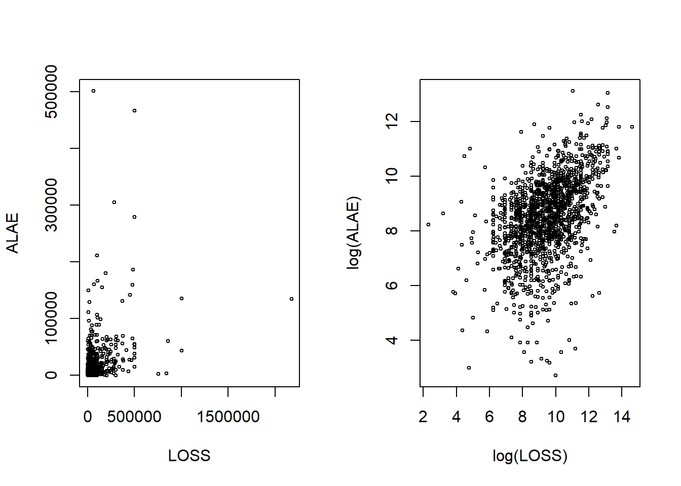
Figure 14.2: Scatter Plot of LOSS and ALAE
R Code for Loss versus Expense Scatterplots
14.4.2 Marginal Models
We first examine the marginal distributionsThe probability distribution of the variables contained in the subset of a collection of random variables of losses and expenses before going through the joint modeling. The histograms show that both \({\tt LOSS}\) and \({\tt ALAE}\) are right-skewed and fat-tailedA fat-tailed distribution is a probability distribution that exhibits a large skewness or kurtosis, relative to that of either a normal distribution or an exponential distribution. Because of these features, for both marginal distributions of losses and expenses, we consider a Pareto distribution, distribution function of the form
\[ F(y)=1- \left( 1 + \frac{\theta}{y+ \theta} \right) ^{\alpha}. \]
Here, \(\theta\) is a scale parameter and \(\alpha\) is a shape parameter. Section 18.2 provides details of this distribution.
The marginal distributions of losses and expenses are fit using the method of maximum likelihood. Specifically, we use the vglm function from the R VGAM package. Firstly, we fit the marginal distribution of \({\tt ALAE}\). Parameters are summarized in Table 14.6.
R Code for Pareto Fitting of ALAE
We repeat this procedure to fit the marginal distribution of the \({\tt LOSS}\) variable. Because the loss variable also seems right-skewed and heavy-tailed data, we also model the marginal distribution with the Pareto distribution (although with different parameters).
R Code for Pareto Fitting of LOSS
Table 14.6. Summary of Pareto Maximum Likelihood Fitted Parameters from the LGPIF Data
\[ {\small \begin{matrix} \begin{array}{l|r|r} \hline & \text{Shape } \hat{\theta} &\text{Scale } \hat{\alpha} \\ \hline ALAE & 15133.60360 & 2.22304 \\ LOSS & 16228.14797 & 1.23766 \\ \hline \end{array} \end{matrix}} \]
To visualize the fitted distribution of \({\tt LOSS}\) and \({\tt ALAE}\) variables, one can use the estimated parameters and plot the corresponding distribution function and density function. For more details on the selection of marginal models, see Chapter 4.
14.4.3 Probability Integral Transformation
When studying simulation, in Section 6.1.2 we learned about the inverse transform methodSamples a uniform number between 0 and 1 to represent the randomly selected percentile, then uses the inverse of the cumulative density function of the desired distribution to simulate from in order to find the simulated value from the desired distribution. This is a way of mapping a \(U(0,1)\) random variable into a random variable \(X\) with distribution function \(F\) via the inverse of the distribution, that is, \(X = F^{-1}(U)\). The probability integral transformationAny continuous variable can be mapped to a uniform random variable via its distribution function goes in the other direction, it states that \(F(X) = U\). Although the inverse transform result is available when the underlying random variable is continuous, discrete or a hybrid combination of the two, the probability integral transform is mainly useful when the distribution is continuous. That is the focus of this chapter.
We use the probability integral transform for two purposes: (1) for diagnostic purposes, to check that we have correctly specified a distribution function and (2) as an input into the copula function in equation (14.1).
For the first purpose, we can check to see whether the Pareto is a reasonable distribution to model our marginal distributions. Given the fitted Pareto distribution, the variable \({\tt ALAE}\) is transformed to the variable \(u_1\), which follows a uniform distribution on \([0,1]\):
\[ u_1 = \hat{F}_{1}^{-1}(ALAE) = 1 - \left( 1 + \frac{ALAE}{\hat{\theta}} \right)^{-\hat{\alpha}}. \]
After applying the probability integral transformation to the \({\tt ALAE}\) variable, we plot the histogram of Transformed \({\tt ALAE}\) in Figure 14.3. This plot appears reasonably close to what we expect to see with a uniform distribution, suggesting that the Pareto distribution is a reasonable specification.
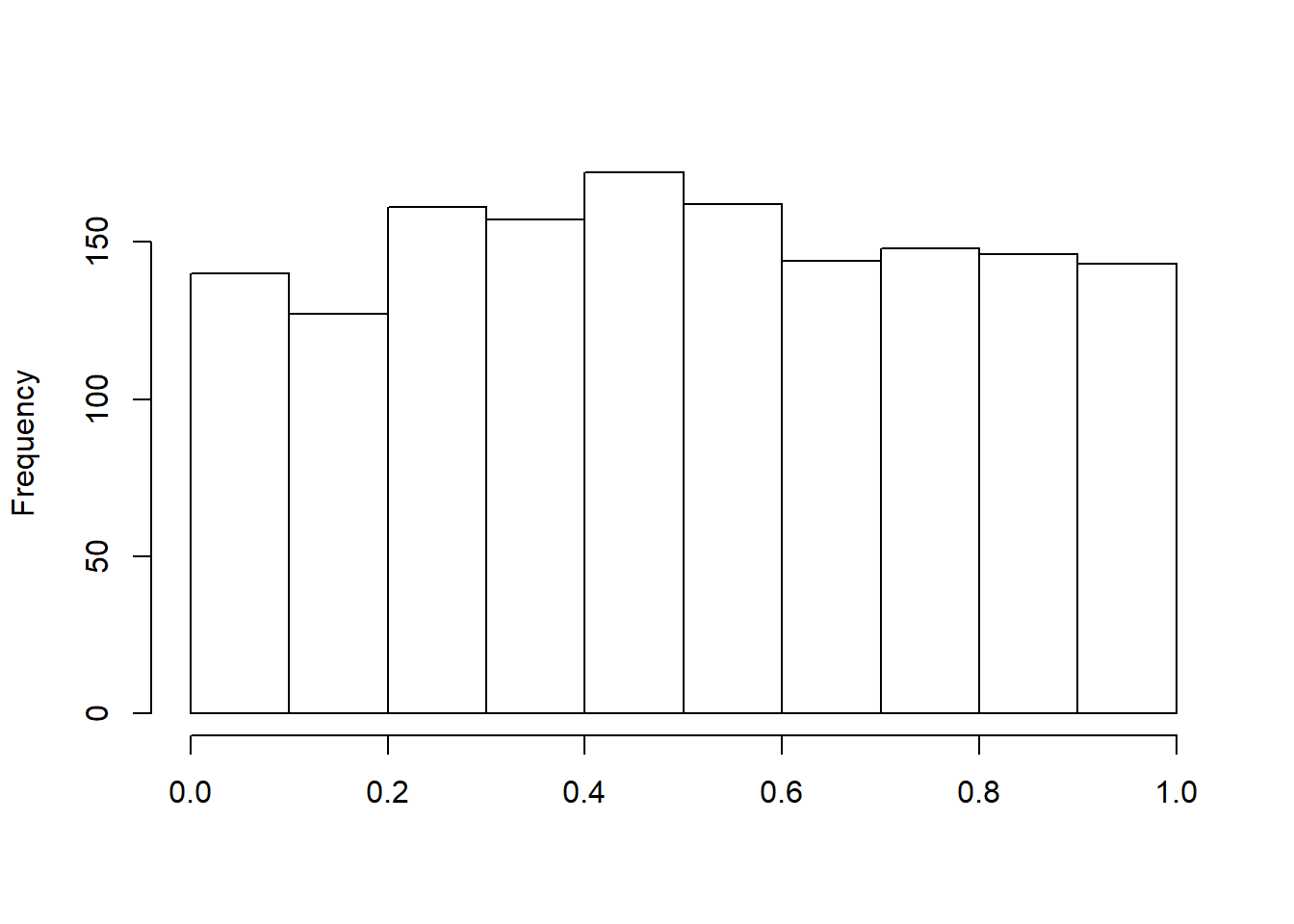
Figure 14.3: Histogram of Transformed ALAE
In the same way, the variable \({\tt LOSS}\) is also transformed to the variable \(u_2\), which follows a uniform distribution on \([0,1]\). The left-hand panel of Figure 14.4 shows a plot the histogram of Transformed \({\tt ALAE}\), again reinforcing the Pareto distribution specification. For another way of looking at the data, the variable \(u_2\) can be transformed to a normal score with the quantile function of standard normal distribution. As we see in Figure 14.4, normal scores of the variable \({\tt LOSS}\) are approximately marginally standard normal. This figure is helpful because analysts are used to looking for patterns of approximate normality (which seems to be evident in the figure). The logic is that, if the Pareto distribution is correctly specified, then transformed losses \(u_2\) should be approximately normal, and the normal scores \(\Phi^{-1}(u_2)\), should be approximately normal. (Here, \(\Phi\) is the cumulative standard normal distribution function.)
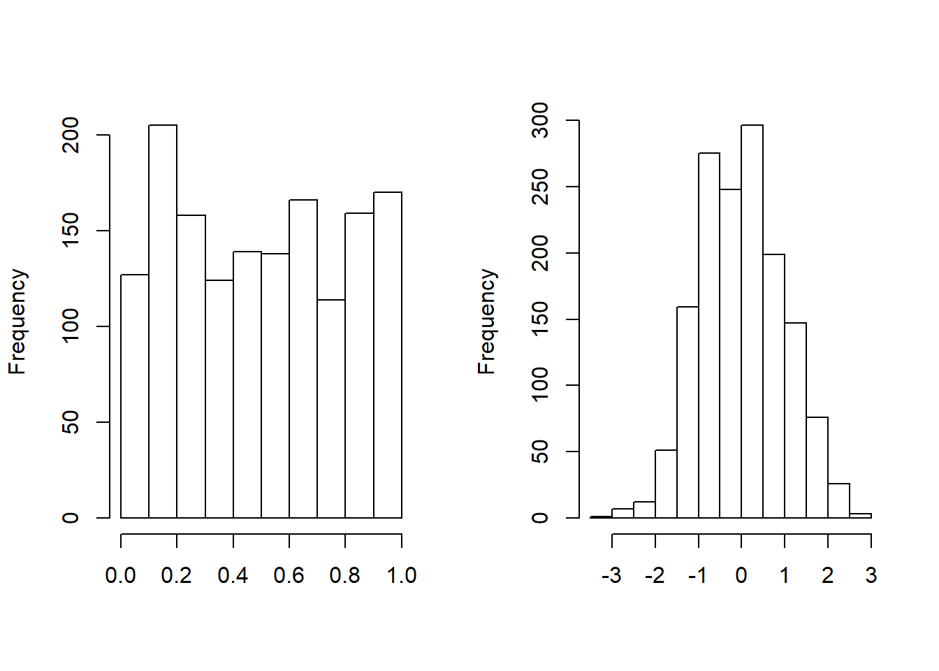
Figure 14.4: Histogram of Transformed Loss. The left-hand panel shows the distribution of probability integral transformed losses. The right-hand panel shows the distribution for the corresponding normal scores.
R Code for Histograms of Transformed Variables
14.4.4 Joint Modeling with Copula Function
Before jointly modeling losses and expenses, we draw the scatterplot of transformed variables \((u_1, u_2)\) and the scatterplot of normal scores in Figure 14.5. The left-hand panel is a plot of \(u_1\) versus \(u_2\), where \(u_1 = \hat{F}_1(ALAE)\) and \(u_2=\hat{F}_2(LOSS)\)). Then we transform each one using an inverse standard normal distribution function, \(\Phi^{-1}(\cdot)\), or qnorm in R to get normal scores. As in Figure 14.2, it is difficult to see patterns in the left-hand panel. However, with rescaling, patterns are evident in the right-hand panel. To learn more details about normal scores and their applications in copula modeling, see Joe (2014).
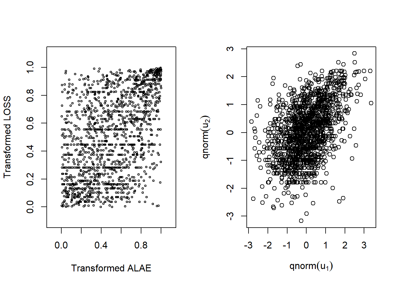
Figure 14.5: Left: Scatter plot for transformed variables. Right:Scatter plot for normal scores
R Code for Scatter Plots and Correlation
The right-hand panel of Figure 14.2 shows us there is a positive dependency between these two random variables. This can be summarized using, for example, Spearman’s rho that turns out to be 0.451. As we learned in Section 14.2.2.1, this statistics depends only on the order of the two variables through their respective ranks. Therefore, the statistic is the same for (1) the original data in Figure 14.2, (2) the data transformed to uniform scales in the left-hand panel of Figure 14.5, and (3) the normal scores in the right-hand panel of Figure 14.5.
The next step is to calculate estimates of the copula parameters. One option is to use traditional maximum likelihood and determine all the parameters at the same time which can be computationally burdensome. Even in our simple example, this means maximizing a (log) likelihood function over five parameters, two for the marginal \({\tt ALAE}\) distribution, two for the marginal \({\tt LOSS}\) distribution, and one for the copula. A widely alternative, known as the inference for margins (IFM) approach, is to simply use the fitted marginal distributions, \(u_1\) and \(u_2\), as inputs when determining the copula. This is the approach taken here. In the following code, you will see that it turns how that the fitted copula parameter \(\hat{\gamma} = 3.114\).
R Code for IFM Fitting with Frank’s Copula
To visualize the fitted Frank’s copula, the distribution function and density function perspective plots are drawn in Figure 14.6.
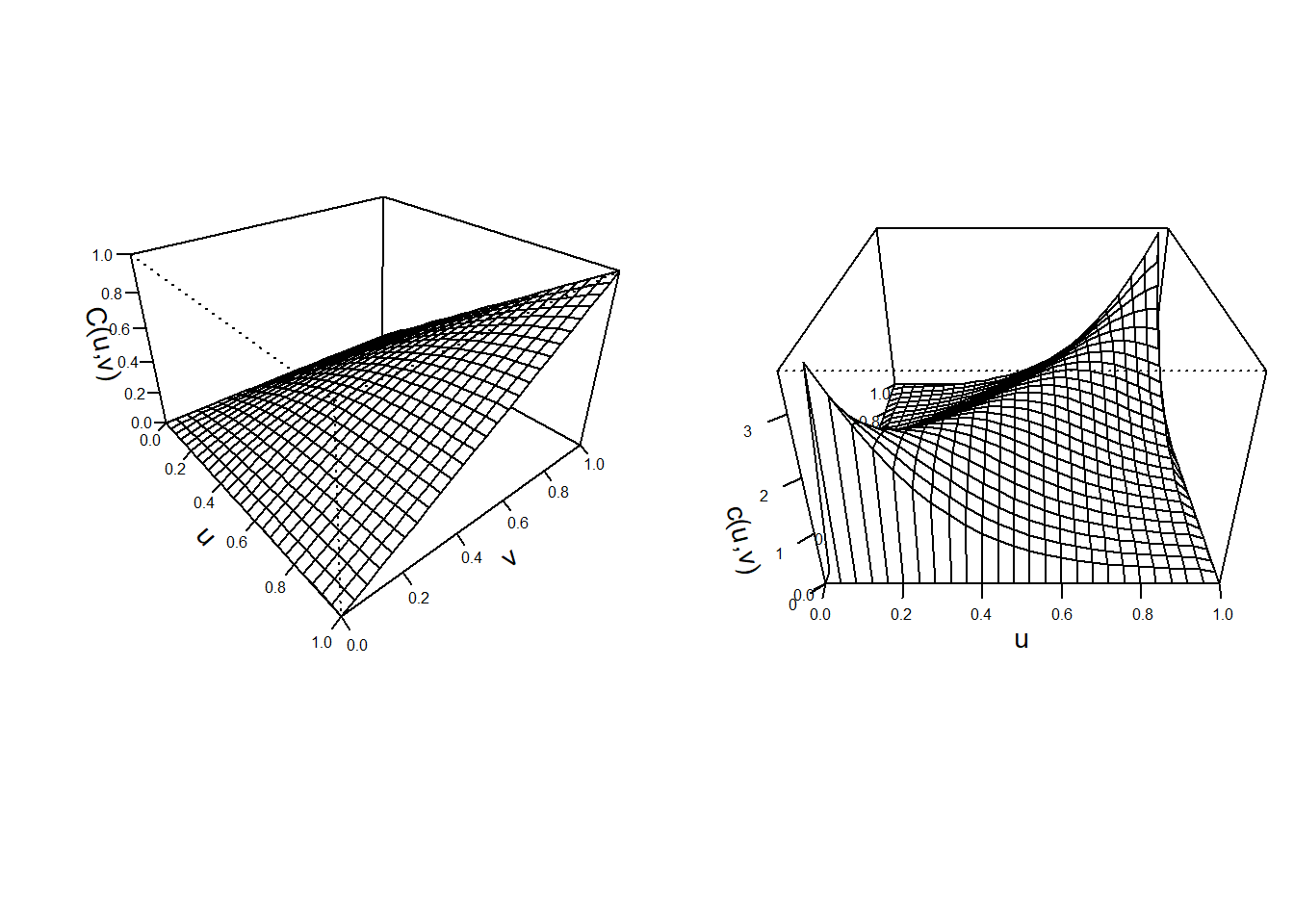
Figure 14.6: Left: Plot for distribution function for Franks Copula. Right:Plot for density function for Franks Copula
R Code for Frank’s Copula Plots
14.5 Types of Copulas
In this section, you learn how to:
- Define the basic types of copulas, including the normal, \(t\)-, elliptical, and Archimedean copulas
- Interpret bounds that limit copula distribution functions as the amount of dependence varies
- Calculate measures of association for different copulas and interpret their properties
- Interpret tail dependency for different copulas
There are several families of copulas have been described in the literature. Two main families of the copula families are the Archimedean and Elliptical copulas.
14.5.1 Normal (Gaussian) Copulas
We started our study with Frank’s copula in equation (14.2) because it can capture both positive and negative dependence and has a readily understood analytic form. However, extensions to multivariate cases where \(p>2\) are not easy and so we look to alternatives. In particular, the normal, or Gaussian, distribution has been used for many years in empirical work, starting with Gauss in 1887. So, it is natural to turn to this distribution as a benchmark for understanding multivariate dependencies.
For a multivariate normal distribution, think of \(p\) normal random variables, each with mean zero and standard deviation one. Their dependence is controlled by \(\boldsymbol \Sigma\), a correlation matrixA table showing correlation coefficients between variables, with ones on the diagonal. The number in the \(i\)th row and \(j\)th column, say \(\boldsymbol \Sigma_{ij}\), gives the correlation between the \(i\)th and \(j\)th normal random variables. This collection of random variables has a multivariate normal distribution with probability density function
\[\begin{equation} \phi_N (\mathbf{z})= \frac{1}{(2 \pi)^{p/2}\sqrt{\det \boldsymbol \Sigma}} \exp\left( -\frac{1}{2} \mathbf{z}^{\prime} \boldsymbol \Sigma^{-1}\mathbf{z}\right). \tag{14.3} \end{equation}\]
To develop the corresponding copula version, it is possible to start with equation (14.1), evaluate this using normal variables, and go through a bit of calculus. Instead, we simply state as a definition, the normal (Gaussian) copula density function is
\[ c_N(u_1, \ldots, u_p) = \phi_N \left(\Phi^{-1}(u_1), \ldots, \Phi^{-1}(u_p) \right) \prod_{j=1}^p \frac{1}{\phi(\Phi^{-1}(u_j))}. \]
Here, we use \(\Phi\) and \(\phi\) to denote the standard normal distribution and density functions. Unlike the usual probability density function \(\phi_N\), the copula density function has its domain on the hyper-cube \([0,1]^p\). For contrast, Figure 14.7 compares these two density functions.
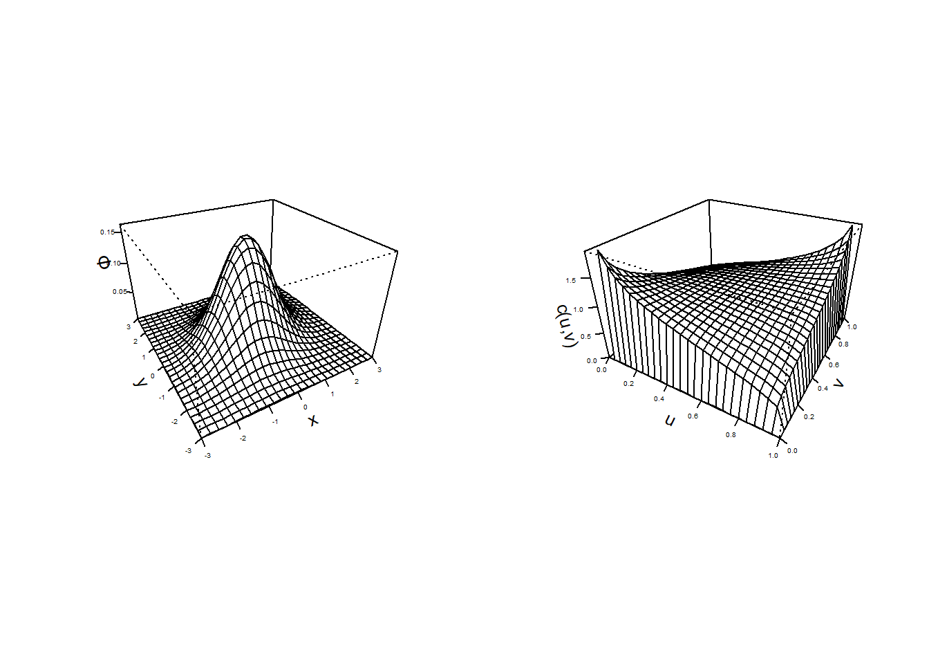
Figure 14.7: Bivariate Normal Probability Density Function Plots. The left-hand panel is a traditional bivariate normal probability density function. The right-hand plot is a plot of the copula density for the normal distribution.
R Code for Normal pdf and Normal Copula pdf Plots
14.5.2 t- and Elliptical Copulas
Another copula used widely in practice is the \(t\)- copula. Both the \(t\)- and the normal copula are special cases of a family known as elliptical copulas, so we introduce this general family first, then specialize to the case of the \(t\)- copula.
The normal and the \(t\)- distributions are examples of symmetric distributions. More generally, elliptical distributionsAny member of a broad family of probability distributions that generalize the multivariate normal distribution is a class of distributions that are symmetric and can be multivariate. In short, an elliptical distribution is a type of symmetric, multivariate distribution. The multivariate normal and multivariate \(t\)- are special types of elliptical distributions.
Elliptical copulasThe copulas of elliptical distributions are constructed from elliptical distributions. This copula decomposes a (multivariate) elliptical distribution into their univariate elliptical marginal distributions by Sklar’s theorem. Properties of elliptical copulas can be obtained from the properties of the corresponding elliptical distributions, see for example, Hofert et al. (2018).
In general, a \(p\)-dimensional vector of random variables has an elliptical distribution if the density can be written as
\[ h_E (\mathbf{z})= \frac{k_p}{\sqrt{\det \boldsymbol \Sigma}} g_p \left( \frac{1}{2} (\mathbf{z}- \boldsymbol \mu)^{\prime} \boldsymbol \Sigma^{-1}(\mathbf{z}- \boldsymbol \mu) \right) , \]
for \(\mathbf{z} \in R^p\) and \(k_p\) is a constant, determined so the density integrates to one. The function \(g_p(\cdot)\) is called a generator because it can be used to produce different distributions. Table 14.7 summarizes a few choices used in actuarial practice. The choice \(g_p(x) = \exp(-x)\) gives rises to the normal pdf in equation (14.3). The choice \(g_p(x) = \exp(-(1+2x/r)^{-(p+r)/2})\) gives rise to a multivariate \(t\)- distribution with \(r\) degrees of freedom with pdf
\[ h_{t_r} (\mathbf{z})= \frac{k_p}{\sqrt{\det \boldsymbol \Sigma}} \exp\left[- \left( 1+ \frac{(\mathbf{z}- \boldsymbol \mu)^{\prime} \boldsymbol \Sigma^{-1}(\mathbf{z}- \boldsymbol \mu)}{r} \right)^{-(p+r)/2}\right] . \]
Table 14.7. Generator Functions (\(g_p(\cdot)\)) for Selected Elliptical Distributions
\[ \small\begin{array}{lc} \hline & Generator \\ Distribution & g_p(x) \\ \hline \text{Normal distribution} & e^{-x}\\ t-\text{distribution with }r \text{ degrees of freedom} & (1+2x/r)^{-(p+r)/2}\\ \text{Cauchy} & (1+2x)^{-(p+1)/2}\\ \text{Logistic} & e^{-x}/(1+e^{-x})^2\\ \text{Exponential power} & \exp(-rx^s)\\ \hline \end{array} \]
We can use elliptical distributions to generate copulas. Because copulas are concerned primarily with relationships, we may restrict our considerations to the case where \(\mu = \mathbf{0}\) and \(\boldsymbol \Sigma\) is a correlation matrix. With these restrictions, the marginal distributions of the multivariate elliptical copula are identical; we use \(H\) to refer to this marginal distribution function and \(h\) is the corresponding density. This marginal density is \(h(z) = k_1 g_1(z^2/2).\) For example, in the normal case we have \(H(\cdot)=\Phi(\cdot)\) and \(h(\cdot)=\phi(\cdot)\).
We are now ready to define the pdf of the elliptical copula, a function defined on the unit cube \([0,1]^p\) as
\[ {c}_E(u_1, \ldots, u_p) = h_E \left(H^{-1}(u_1), \ldots, H^{-1}(u_p) \right) \prod_{j=1}^p \frac{1}{h(H^{-1}(u_j))}. \]
As noted above, most empirical work focuses on the normal copula and \(t\)-copula. Specifically, \(t\)-copulas are useful for modeling the dependency in the tails of bivariate distributions, especially in financial risk analysis applications. The \(t\)-copulas with same association parameter in varying the degrees of freedom parameter show us different tail dependency structures. For more information on about \(t\)-copulas readers can see Joe (2014) and Hofert et al. (2018).
14.5.3 Archimedean Copulas
This class of copulas is also constructed from a generator function. For Archimedean copulas, we assume that \(g(\cdot)\) is a convex, decreasing function with domain [0,1] and range \([0, \infty)\) such that \(g(0)=0\). Use \(g^{-1}\) for the inverse function of \(g\). Then the function
\[ C_g(u_1, \ldots, u_p) = g^{-1} \left(g(u_1)+ \cdots + g(u_p) \right) \]
is said to be an Archimedean copula distribution function.
For the bivariate case, \(p=2\), an Archimedean copula function can be written by the function
\[ C_{g}(u_1, \, u_2) = g^{-1} \left(g(u_1) + g(u_2) \right). \]
Some important special cases of Archimedean copulas include the Frank, Clayton/Cook-Johnson, and Gumbel/Hougaard copulas. Each copula class is derived from different generator functions. As another useful special case, recall the Frank’s copula described in Sections 14.3 and 14.4. To illustrate, we now provide explicit expressions for the Clayton and Gumbel/Hougaard copulas.
Clayton Copula
For \(p=2\), the Clayton copula is parameterized by \(\gamma \in [-1,\infty)\) is defined by
\[ C_{\gamma}^C(u)=\max\{u_1^{-\gamma}+u_2^{-\gamma}-1,0\}^{1/\gamma}, \quad u \in [0,1]^2. \]
This is a bivariate distribution function defined on the unit square \([0,1]^2.\) The range of dependence is controlled by the parameter \(\gamma\), similar to Frank’s copula.
Gumbel-Hougaard Copula
The Gumbel-Hougaard copula is parametrized by \(\gamma \in [1,\infty)\) and defined by
\[ C_{\gamma}^{GH}(u)=\exp\left(-\left(\sum_{i=1}^2 (-\log u_i)^{\gamma}\right)^{1/\gamma}\right), \quad u\in[0,1]^2. \]
For more information on Archimedean copulas, see Joe (2014), Frees and Valdez (1998), and Genest and Mackay (1986).
14.5.4 Properties of Copulas
With many choices of copulas available, it is helpful for analysts to understand general features of how these alternatives behave.
14.5.4.1 Bounds on Association
Any distribution function is bounded below by zero and from above by one. Additional types of bounds are available in multivariate contexts. These bounds are useful when studying dependencies. That is, as an analyst thinks about variables as being extremely dependent, one has available bounds that cannot be exceeded, regardless of the dependence. The most widely used bounds in dependence modeling are known as the Fréchet-Höeffding bounds, given as
\[ \max( u_1 +\cdots+ u_p + p -1, 0) \leq C(u_1, \ldots, u_p) \leq \min (u_1, \ldots,u_p). \]
To see the right-hand side of this equation, note that
\[ C(u_1,\ldots, u_p) = \Pr(U_1 \leq u_1, \ldots, U_p \leq u_p) \leq \Pr(U_j \leq u_j), \]
for \(j=1,\ldots,p\). The bound is achieved when \(U_1 = \cdots = U_p\). To see the left-hand side when \(p=2\), consider \(U_2=1-U_1\). In this case, if \(1-u_2 < u_1\) then \[ \Pr(U_1 \leq u_1, U_2 \leq u_2) = \Pr ( 1-u_2 \leq U_1 < u_1) =u_1+u_2-1. \] See, for example, Nelson (1997) for additional discussion.
To see how these bounds relate to the concept of dependence, consider the case of \(p=2\). As a benchmark, first note that the product copula is \(C(u_1,u_2)=u_1 \cdot u_2\) is the result of assuming independence between random variables. Now, from the above discussion, we see that the lower bound is achieved when the two random variables are perfectly negatively related (\(U_2=1-U_1\)). Further, it is clear that the upper bound is achieved when they are perfectly positively related (\(U_2=U_1\)). To emphasize this, the Frechet-Hoeffding boundsBounds of multivariate distribution functions for two random variables appear in Figure 14.8.
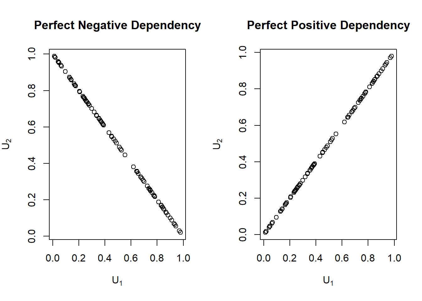
Figure 14.8: Perfect Positive and Perfect Negative Dependence Plots
R Code for the Fréchet-Höeffding Bounds for Two Random Variables
14.5.4.2 Measures of Association
Empirical versions of Spearman’s rho and Kendall’s tau were introduced in Sections 14.2.2.1 and 14.2.2.2, respectively. The interesting thing about these expressions is that these summary measures of association are based only on the ranks of each variable. Thus, any strictly increasing transform does not affect these measures of association. Specifically, consider two random variables, \(Y_1\) and \(Y_2\), and let m\(_1\) and m\(_2\) be strictly increasing functions. Then, the association, when measured by Spearman’s rho or Kendall’s tau, between \(m_1(Y_1)\) and \(m_2(Y_2)\) does not change regardless of the choice of m\(_1\) and m\(_2\). For example, this allows analysts to consider dollars, Euros, or log dollars, and still retain the same essential dependence. As we have seen in Section 14.2, this is not the case with the Pearson’s measure of correlation.
Schweizer, Wolff, and others (1981) established that the copula accounts for all the dependence in the sense that they way \(Y_1\) and \(Y_2\) “move together” is captured by the copula, regardless of the scale in which each variable is measured. They also showed that (population versions of) the two standard nonparametric measures of association could be expressed solely in terms of the copula function. Spearman’s correlation coefficient is given by
\[\begin{equation} \rho_S = 12 \int_0^1 \int_0^1 \left\{C(u,v) - uv \right\} du dv. \tag{14.4} \end{equation}\]
Kendall’s tau is given by
\[ \tau= 4 \int_0^1 \int_0^1 C(u,v)~dC(u,v) - 1 . \]
For these expressions, we assume that \(Y_1\) and \(Y_2\) have a jointly continuous distribution function.
Example. Loss versus Expenses. Earlier, in Section 14.4, we saw that the Spearman’s correlation was 0.452, calculated with the rho function. Then, we fit Frank’s copula to these data, and estimated the dependence parameter to be \(\hat{\gamma} = 0.452\). As an alternative, the following code shows how to use the empirical version of equation (14.4). In this case, the Spearman’s correlation coefficient is 0.462, which is close to the sample Spearman’s correlation coefficient, 0.452.
R Code for Spearman’s Correlation Using Frank’s Copula
14.5.4.3 Tail Dependency
There are applications in which it is useful to distinguish the part of the distribution in which the association is strongest. For example, in insurance it is helpful to understand association among the largest losses, that is, association in the right tails of the data.
To capture this type of dependency, we use the right-tail concentration function, defined as
\[ R(z) = \frac{\Pr(U_1 >z, U_2 > z)}{1-z} =\Pr(U_1 > z | U_2 > z) =\frac{1 - 2z + C(z,z)}{1-z} . \]
As a benchmark, \(R(z)\) will be equal to \(z\) under independence. Joe (1997) uses the term “upper tail dependence parameter” for \(R = \lim_{z \rightarrow 1} R(z)\).
In the same way, one can define the left-tail concentration function as
\[ L(z) = \frac{\Pr(U_1 \leq z, U_2 \leq z)}{z}=\Pr(U_1 \leq z | U_2 \leq z) =\frac{ C(z,z)}{z}, \]
with the lower tail dependence parameter \(L = \lim_{z \rightarrow 0} L(z)\). A tail dependencyA measure of their comovements in the tails of the distributions concentration function captures the probability of two random variables simultaneously having extreme values.
It is of interest to see how well a given copula can capture tail dependence. To this end, we calculate the left and right tail concentration functions for four different types of copulas; Normal, Frank, Gumbel and \(t\)- copulas. The results are summarized for concentration function values for these four copulas in Table 14.8. As in Venter (2002), we show \(L(z)\) for \(z\leq 0.5\) and \(R(z)\) for \(z>0.5\) in the tail dependence plot in Figure 14.9. We interpret the tail dependence plot to mean that both the Frank and Normal copula exhibit no tail dependence whereas the \(t\)- and the Gumbel do so. The \(t\)- copula is symmetric in its treatment of upper and lower tails.
Table 14.8. Tail Dependence Parameters for Four Copulas
\[ {\small \begin{matrix} \begin{array}{l|rr} \hline \text{Copula} & \text{Lower} & \text{Upper} \\ \hline \text{Frank} & 0 & 0 \\ \text{Gumbel} & 0 & 0.74 \\ \text{Normal} & 0 & 0 \\ t- & 0.10 & 0.10 \\ \hline \end{array} \end{matrix}} \]
R Code for Tail Copula Functions for Different Copulas
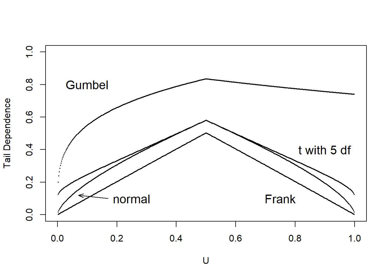
Figure 14.9: Tail Dependence Plots
R Code for Tail Dependence Plot for Different Copulas
Show Quiz Solution
14.6 Why is Dependence Modeling Important?
Dependence modeling is important because it enables us to understand the dependence structure by defining the relationship between variables in a dataset. In insurance, ignoring dependence modeling may not impact pricing but could lead to misestimation of required capital to cover losses. For instance, from Section 14.4 , it is seen that there was a positive relationship between \({\tt LOSS}\) and \({\tt ALAE}\). This means that, if there is a large loss then we expect expenses to be large as well and ignoring this relationship could lead to mis-estimation of reserves.
To illustrate the importance of dependence modeling, we refer you back to portfolio management example in Section 10.4.3.3 that assumed that the property and liability risks are independent. Now, we incorporate dependence by allowing the four lines of business to depend on one another through a Gaussian copula. In Table 14.9, we show that dependence affects the portfolio quantiles (\(VaR_q\)), although not the expected values. For instance, the \(VaR_{0.99}\) for total risk which is the amount of capital required to ensure, with a \(99\%\) degree of certainty that the firm does not become technically insolvent is higher when we incorporate dependence. This leads to less capital being allocated when dependence is ignored and can cause unexpected solvency problems.
Table 14.9. Results for Portfolio Expected Value and Quantiles (\(VaR_q\))
\[ {\small \begin{matrix} \begin{array}{l|rrrr} \hline \text{Independent} &\text{Expected} & VaR_{0.9} & VaR_{0.95} & VaR_{0.99} \\ &\text{Value} & & & \\ \hline \text{Retained} & 269 & 300 & 300 & 300 \\ \text{Insurer} & 2,274 & 4,400 & 6,173 & 11,859 \\ \text{Total} & 2,543 & 4,675 & 6,464 & 12,159 \\ \hline \text{Gaussian Copula}&\text{Expected}& VaR_{0.9} & VaR_{0.95} & VaR_{0.99} \\ &\text{Value} & & & \\ \hline \text{Retained} & 269 & 300 & 300 & 300 \\ \text{Insurer} & 2,340 & 4,988 & 7,339 & 14,905 \\ \text{Total} & 2,609 & 5,288 & 7,639 & 15,205 \\ \hline \end{array} \end{matrix}} \]
R Code for Simulation Using Gaussian Copula
Show Quiz Solution
14.7 Further Resources and Contributors
Contributors
- Edward W. (Jed) Frees and Nii-Armah Okine, University of Wisconsin-Madison, and Emine Selin Sarıdaş, Mimar Sinan University, are the principal authors of the initial version of this chapter. Email: jfrees@bus.wisc.edu for chapter comments and suggested improvements.
- Chapter reviewers include: Runhuan Feng, Fei Huang, Himchan Jeong, Min Ji, and Toby White.
TS 14.A. Other Classic Measures of Scalar Associations
TS 14.A.1. Blomqvist’s Beta
Blomqvist (1950) developed a measure of dependence now known as Blomqvist’s betaA dependence measure based on the center of the distribution, also called the median concordance coefficient and the medial correlation coefficient. Using distribution functions, this parameter can be expressed as
\[\begin{equation*} \beta_B = 4F\left(F^{-1}_X(1/2),F^{-1}_Y(1/2) \right) - 1. \end{equation*}\]
That is, first evaluate each marginal at its median (\(F^{-1}_X(1/2)\) and \(F^{-1}_Y(1/2)\), respectively). Then, evaluate the bivariate distribution function at the two medians. After rescaling (multiplying by 4 and subtracting 1), the coefficient turns out to have a range of \([-1,1]\), where 0 occurs under independence.
Like Spearman’s rho and Kendall’s tau, an estimator based on ranks is easy to provide. First write \(\beta_B = 4C(1/2,1/2)-1 = 2\Pr((U_1-1/2)(U_2-1/2))-1\) where \(U_1, U_2\) are uniform random variables. Then, define
\[ \hat{\beta}_B = \frac{2}{n} \sum_{i=1}^n I\left( (R(X_{i})-\frac{n+1}{2})(R(Y_{i})-\frac{n+1}{2}) \ge 0 \right)-1 . \]
See, for example, Joe (2014), page 57 or Hougaard (2000), page 135, for more details.
Because Blomqvist’s parameter is based on the center of the distribution, it is particularly useful when data are censored; in this case, information in extreme parts of the distribution are not always reliable. How does this affect a choice of association measures? First, recall that association measures are based on a bivariate distribution function. So, if one has knowledge of a good approximation of the distribution function, then calculation of an association measure is straightforward in principle. Second, for censored data, bivariate extensions of the univariate Kaplan-Meier distribution function estimator are available. For example, the version introduced in Dabrowska (1988) is appealing. However, because of instances when large masses of data appear at the upper range of the data, this and other estimators of the bivariate distribution function are unreliable. This means that, summary measures of the estimated distribution function based on Spearman’s rho or Kendall’s tau can be unreliable. For this situation, Blomqvist’s beta appears to be a better choice as it focuses on the center of the distribution. Hougaard (2000), Chapter 14, provides additional discussion.
You can obtain the Blomqvist’s beta, using the betan() function from the copula library in R. From below, \(\beta_B=0.3\) between the \({\tt Coverage}\) rating variable in millions of dollars and \({\tt Claim}\) amount variable in dollars.
R Code for Blomqvist’s Beta
In addition, to show that the Blomqvist’s beta is invariant under strictly increasing transformations, \(\beta_B=0.3\) between the \({\tt Coverage}\) rating variable in logarithmic millions of dollars and \({\tt Claim}\) amount variable in dollars.
TS 14.A.2. Nonparametric Approach Using Spearman Correlation with Tied Ranks
For the first variable, the average rank of observations in the \(s\)th row is
\[\begin{equation*} r_{1s} = n_{m_1\cdot}+ \cdots+ n_{s-1,\cdot}+ \frac{1}{2} \left(1+ n_{s\cdot}\right) \end{equation*}\] and similarly \(r_{2t} = \frac{1}{2} \left[(n_{\cdot m_1}+ \cdots+ n_{\cdot,s-1}+1)+ (n_{\cdot m_1}+ \cdots+ n_{\cdot s})\right]\). With this, we have Spearman’s rho with tied rank is \[\begin{equation*} \hat{\rho}_S = \frac{\sum_{s=m_1}^{m_2} \sum_{t=m_1}^{m_2} n_{st}(r_{1s} - \bar{r})(r_{2t} - \bar{r})} {\left[\sum_{s=m_1}^{m_2}n_{s \cdot}(r_{1s} - \bar{r})^2 \sum_{t=m_1}^{m_2} n_{\cdot t}(r_{2t} - \bar{r})^2 \right]^2} \end{equation*}\]
where the average rank is \(\bar{r} = (n+1)/2\).
Click to Show Proof for Special Case: Binary Data.
You can obtain the ties-corrected Spearman correlation statistic \(r_S\) using the cor() function in R and selecting the spearman method. From below \(\hat{\rho}_S=-0.09\).
R Code for Ties-corrected Spearman Correlation
Bibliography
Bishop, Yvonne M., Stephen E. Fienberg, and Paul W. Holland. 1975. Discrete Multivariate Analysis: Theory and Practice. Cambridge [etc.]: MIT.
Blomqvist, Nils. 1950. “On a Measure of Dependence Between Two Random Variables.” The Annals of Mathematical Statistic, 593–600.
Dabrowska, Dorota M. 1988. “Kaplan-Meier Estimate on the Plane.” The Annals of Statistics, 1475–89.
Fechner, G. T. 1897. “Kollektivmasslehre.” Wilhelm Englemann, Leipzig.
Frank, Maurice J. 1979. “On the Simultaneous Associativity of F(x, Y) and X+y-F(x, Y).” Aequationes Mathematicae 19 (1): 194–226.
Frees, Edward W., and Emiliano A. Valdez. 1998. “Understanding Relationships Using Copulas.” North American Actuarial Journal 2 (01): 1–25.
Genest, Christian, and Josh Mackay. 1986. “The Joy of Copulas: Bivariate Distributions with Uniform Marginals.” The American Statistician 40: 280–83.
Genest, Christian, and Johanna Nešlohva. 2007. “A Primer on Copulas for Count Data.” Journal of the Royal Statistical Society, 475–515.
Hettmansperger, T. P. 1984. Statistical Inference Based on Ranks. Wiley.
Hofert, Marius, Ivan Kojadinovic, Martin Mächler, and Jun Yan. 2018. Elements of Copula Modeling with R. Springer.
Hougaard, P. 2000. Analysis of Multivariate Survival Data. Springer New York.
Joe, Harry. 2014. Dependence Modeling with Copulas. CRC Press.
Kendall, Maurice G. 1938. “A New Measure of Rank Correlation.” Biometrika, 81–93.
Kendall, M. G. 1945. “The Treatment of Ties in Ranking Problems.” Biometrika 33(3): 239–51.
Lee Rodgers, J, and W. A Nicewander. 1998. “Thirteen Ways to Look at the Correlation Coeffeicient.” The American Statistician 42 (01): 59–66.
Nelson, Roger B. 1997. An Introduction to Copulas. Lecture Notes in Statistics 139.
Schweizer, Berthold, Edward F Wolff, and others. 1981. “On Nonparametric Measures of Dependence for Random Variables.” The Annals of Statistics 9 (4): 879–85.
Sklar, M. 1959. “Fonctions de Repartition a N Dimensions et Leurs Marges.” Publ. Inst. Statist. Univ. Paris 8: 229–31.
Spearman, C. 1904. “The Proof and Measurement of Association Between Two Things.” The American Journal of Psychology 15 (01): 72–101.
Venter, Gary G. 2002. “Tails of Copulas.” In Proceedings of the Casualty Actuarial Society, 89:68–113. 171.
Yule, G. Udny. 1900. “On the Association of Attributes in Statistics: With Illustrations from the Material of the Childhood Society.” Philosophical Transactions of the Royal Society of London. Series A, Containing Papers of a Mathematical or Physical Character, 257–319.
Yule, G. 1912. “On the Methods of Measuring Association Between Two Attributes.” Journal of the Royal Statistical Society, 579–652.