Chapter 6 Simulation and Resampling
Chapter Preview. Simulation is a computationally intensive method used to solve difficult problems. Instead of creating physical processes and experimenting with them in order to understand their operational characteristics, a simulation study is based on a computer representation - it considers various hypothetical conditions as inputs and summarizes the results. Through simulation, a vast number of hypothetical conditions can be quickly and inexpensively examined. Section 6.1 introduces simulation, a wonderful computational tool that is especially useful in complex, multivariate settings.
We can also use simulation to draw from an empirical distribution - this process is known as resampling. Resampling allows us to assess the uncertainty of estimates in complex models. Section 6.2 introduces resampling in the context of bootstrapping to determine the precision of estimators.
Subsequent sections introduce other topics in resampling. Section 6.3 on cross-validation shows how to use it for model selection and validation. Section 6.4 on importance sampling describes resampling in specific regions of interest, such as long-tailed actuarial applications. Section 6.5 on Monte Carlo Markov Chain (MCMC) introduces the simulation and resampling engine underpinning much of modern Bayesian analysis.
6.1 Simulation Fundamentals
In this section, you learn how to:
- Generate approximately independent realizations that are uniformly distributed
- Transform the uniformly distributed realizations to observations from a probability distribution of interest
- Calculate quantities of interest and determine the precision of the calculated quantities
6.1.1 Generating Independent Uniform Observations
The simulationsA computer generation of various hypothetical conditions and outputs, based on the model structure provided that we consider are generated by computers. A major strength of this approach is that they can be replicated, allowing us to check and improve our work. Naturally, this also means that they are not really random. Nonetheless, algorithms have been produced so that results appear to be random for all practical purposes. Specifically, they pass sophisticated tests of independence and can be designed so that they come from a single distribution - our iidIndependent and identically distributed assumption, identically and independently distributed.
To get a sense as to what these algorithms do, we consider a historically prominent method.
Linear Congruential Generator. To generate a sequence of random numbers, start with \(B_0\), a starting value that is known as a seed. This value is updated using the recursive relationship \[B_{n+1} = (a B_n + c) \text{ modulo }m, ~~ n=0, 1, 2, \ldots .\] This algorithm is called a linear congruential generatorAlgorithm that yields pseudo-randomized numbers calculated using a linear recursive relationship and a starting seed value. The case of \(c=0\) is called a multiplicative congruential generator; it is particularly useful for really fast computations.
For illustrative values of \(a\) and \(m\), Microsoft’s Visual Basic uses \(m=2^{24}\), \(a=1,140,671,485\), and \(c = 12,820,163\) (see https://en.wikipedia.org/wiki/Linear_congruential_generator). This is the engine underlying the random number generation in Microsoft’s Excel program.
The sequence used by the analyst is defined as \(U_n=B_n/m.\) The analyst may interpret the sequence {\(U_{i}\)} to be (approximately) identically and independently uniformly distributed on the interval (0,1). To illustrate the algorithm, consider the following.
Example 6.1.1. Illustrative Sequence. Take \(m=15\), \(a=3\), \(c=2\) and \(B_0=1\). Then we have:
| step \(n\) | \(B_n\) | \(U_n\) |
|---|---|---|
| 0 | \(B_0=1\) | |
| 1 | \(B_1 =\mod(3 \times 1 +2) = 5\) | \(U_1 = \frac{5}{15}\) |
| 2 | \(B_2 =\mod(3 \times 5 +2) = 2\) | \(U_2 = \frac{2}{15}\) |
| 3 | \(B_3 =\mod(3 \times 2 +2) = 8\) | \(U_3 = \frac{8}{15}\) |
| 4 | \(B_4 =\mod(3 \times 8 +2) = 11\) | \(U_4 = \frac{11}{15}\) |
Sometimes computer generated random results are known as pseudo-random numbersValues that appear random but can be replicated by formula to reflect the fact that they are machine generated and can be replicated. That is, despite the fact that {\(U_{i}\)} appears to be i.i.d, it can be reproduced by using the same seed number (and the same algorithm).
Example 6.1.2. Generating Uniform Random Numbers in R.
The following code shows how to generate three uniform (0,1) numbers in R using the runif command. The set.seed() function sets the initial seed. In many computer packages, the initial seed is set using the system clock unless specified otherwise.
Three Uniform Random Variates
| Uniform |
|---|
| 0.92424 |
| 0.53718 |
| 0.46920 |
The linear congruential generator is just one method of producing pseudo-random outcomes. It is easy to understand and is widely used. The linear congruential generator does have limitations, including the fact that it is possible to detect long-run patterns over time in the sequences generated (recall that we can interpret independence to mean a total lack of functional patterns). Not surprisingly, advanced techniques have been developed that address some of this method’s drawbacks.
6.1.2 Inverse Transform Method
With the sequence of uniform random numbers, we next transform them to a distribution of interest, say \(F\). A prominent technique is the inverse transform methodSamples a uniform number between 0 and 1 to represent the randomly selected percentile, then uses the inverse of the cumulative density function of the desired distribution to simulate from in order to find the simulated value from the desired distribution, defined as
\[ X_i=F^{-1}\left( U_i \right) . \]
Here, recall from Section 4.1.1 that we introduced the inverse of the distribution function, \(F^{-1}\), and referred to it also as the quantile functionInverse function for the cumulative density function which takes a percentile value in [0,1] as the input, and outputs the corresponding value in the distribution. Specifically, it is defined to be
\[ F^{-1}(y) = \inf_x ~ \{ F(x) \ge y \} . \]
Recall that \(\inf\) stands for infimum or the greatest lower boundLargest value that is less than or equal to a specified subset of values/elements. It is essentially the smallest value of x that satisfies the inequality \(\{F(x) \ge y\}\). The result is that the sequence {\(X_{i}\)} is approximately iid with distribution function \(F\) if the {\(U_i\)} are iid with uniform on \((0,1)\) distribution function.
The inverse transform result is available when the underlying random variable is continuous, discrete or a hybrid combination of the two. We now present a series of examples to illustrate its scope of applications.
Example 6.1.3. Generating Exponential Random Numbers. Suppose that we would like to generate observations from an exponential distribution with scale parameter \(\theta\) so that \(F(x) = 1 - e^{-x/\theta}\). To compute the inverse transform, we can use the following steps: \[ \begin{aligned} y = F(x) &\Leftrightarrow y = 1-e^{-x/\theta} \\ &\Leftrightarrow -\theta \ln(1-y) = x = F^{-1}(y) . \end{aligned} \]
Thus, if \(U\) has a uniform (0,1) distribution, then \(X = -\theta \ln(1-U)\) has an exponential distribution with parameter \(\theta\).
The following R code shows how we can start with the same three uniform random numbers as in Example 6.1.2 and transform them to independent exponentially distributed random variables with a mean of 10. Alternatively, you can directly use the rexp function in R to generate random numbers from the exponential distribution. The algorithm built into this routine is different so even with the same starting seed number, individual realizations will differ.
Three Uniform Random Variates
| Uniform | Exponential 1 | Exponential 2 |
|---|---|---|
| 0.92424 | 25.80219 | 3.25222 |
| 0.53718 | 7.70409 | 8.47652 |
| 0.46920 | 6.33362 | 5.40176 |
Example 6.1.4. Generating Pareto Random Numbers. Suppose that we would like to generate observations from a Pareto distribution with parameters \(\alpha\) and \(\theta\) so that \(F(x) = 1 - \left(\frac{\theta}{x+\theta} \right)^{\alpha}\). To compute the inverse transform, we can use the following steps:
\[ \begin{aligned} y = F(x) &\Leftrightarrow 1-y = \left(\frac{\theta}{x+\theta} \right)^{\alpha} \\ &\Leftrightarrow \left(1-y\right)^{-1/\alpha} = \frac{x+\theta}{\theta} = \frac{x}{\theta} +1 \\ &\Leftrightarrow \theta \left((1-y)^{-1/\alpha} - 1\right) = x = F^{-1}(y) .\end{aligned} \]
Thus, \(X = \theta \left((1-U)^{-1/\alpha} - 1\right)\) has a Pareto distribution with parameters \(\alpha\) and \(\theta\).
Inverse Transform Justification. Why does the random variable \(X = F^{-1}(U)\) have a distribution function \(F\)?
Show A Snippet of Theory
We now consider some discrete examples.
Example 6.1.5. Generating Bernoulli Random Numbers. Suppose that we wish to simulate random variables from a Bernoulli distribution with parameter \(q=0.85\).
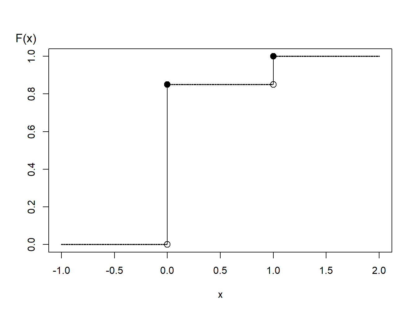
Figure 6.1: Distribution Function of a Binary Random Variable
A graph of the cumulative distribution function in Figure 6.1 shows that the quantile function can be written as \[ \begin{aligned} F^{-1}(y) = \left\{ \begin{array}{cc} 0 & 0<y \leq 0.85 \\ 1 & 0.85 < y \leq 1.0 . \end{array} \right. \end{aligned} \]
Thus, with the inverse transform we may define \[ \begin{aligned} X = \left\{ \begin{array}{cc} 0 & 0<U \leq 0.85 \\ 1 & 0.85 < U \leq 1.0 \end{array} \right. \end{aligned} \] For illustration, we generate three random numbers to get
Three Random Variates
| Uniform | Binary X |
|---|---|
| 0.92424 | 1 |
| 0.53718 | 0 |
| 0.46920 | 0 |
Example 6.1.6. Generating Random Numbers from a Discrete Distribution. Consider the time of a machine failure in the first five years. The distribution of failure times is given as:
Discrete Distribution
| Time | 1.0 | 2.0 | 3.0 | 4.0 | 5.0 |
| Probability | 0.1 | 0.2 | 0.1 | 0.4 | 0.2 |
| Distribution Function | 0.1 | 0.3 | 0.4 | 0.8 | 1.0 |
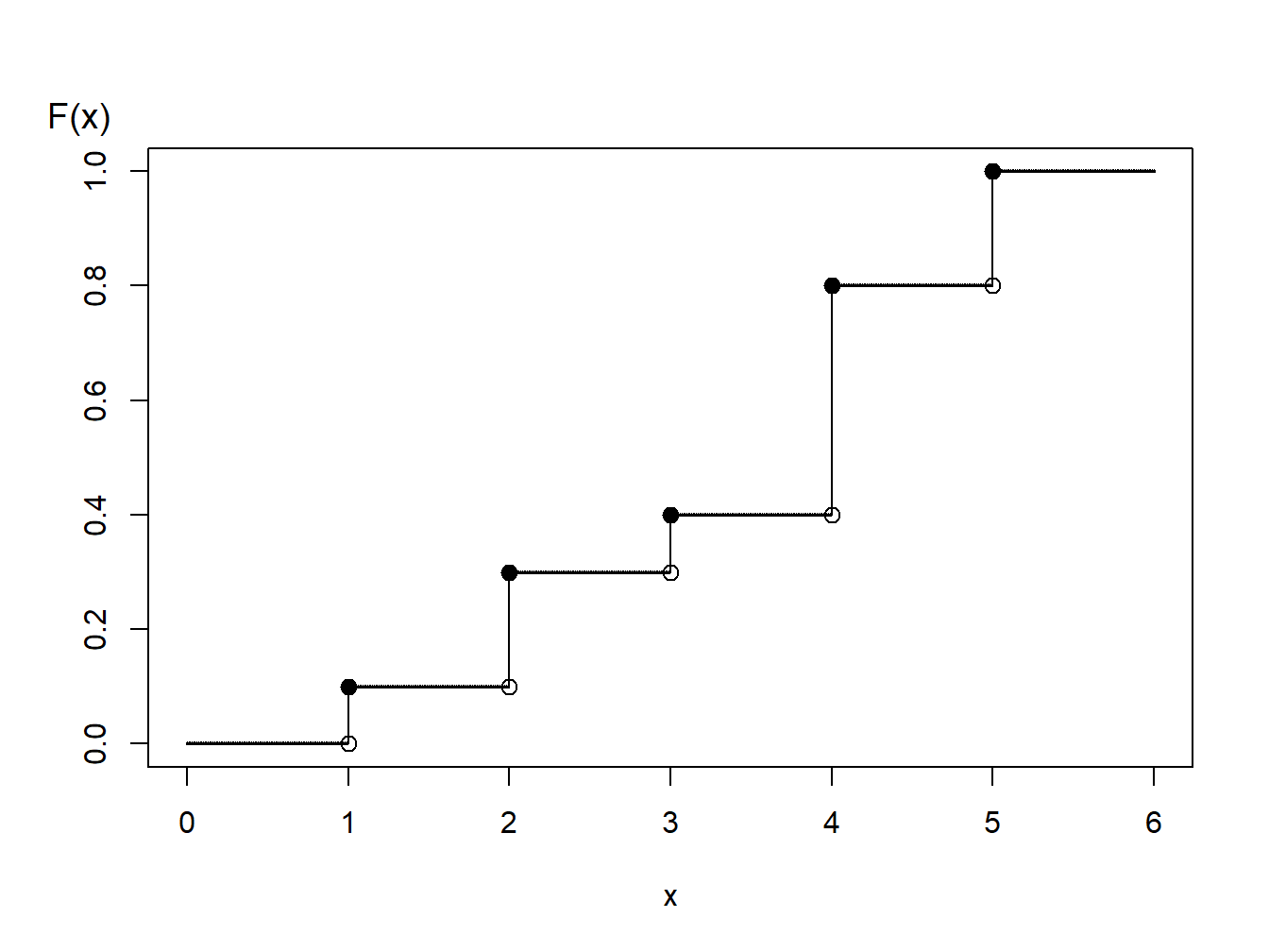
Figure 6.2: Distribution Function of a Discrete Random Variable
Using the graph of the distribution function in Figure 6.2, with the inverse transform we may define
\[ \small{ \begin{aligned} X = \left\{ \begin{array}{cc} 1 & 0<U \leq 0.1 \\ 2 & 0.1 < U \leq 0.3\\ 3 & 0.3 < U \leq 0.4\\ 4 & 0.4 < U \leq 0.8 \\ 5 & 0.8 < U \leq 1.0 . \end{array} \right. \end{aligned} } \]
For general discrete random variables there may not be an ordering of outcomes. For example, a person could own one of five types of life insurance products and we might use the following algorithm to generate random outcomes:
\[ {\small \begin{aligned} X = \left\{ \begin{array}{cc} \textrm{whole life} & 0<U \leq 0.1 \\ \textrm{endowment} & 0.1 < U \leq 0.3\\ \textrm{term life} & 0.3 < U \leq 0.4\\ \textrm{universal life} & 0.4 < U \leq 0.8 \\ \textrm{variable life} & 0.8 < U \leq 1.0 . \end{array} \right. \end{aligned} } \]
Another analyst may use an alternative procedure such as:
\[ {\small \begin{aligned} X = \left\{ \begin{array}{cc} \textrm{whole life} & 0.9<U<1.0 \\ \textrm{endowment} & 0.7 \leq U < 0.9\\ \textrm{term life} & 0.6 \leq U < 0.7\\ \textrm{universal life} & 0.2 \leq U < 0.6 \\ \textrm{variable life} & 0 \leq U < 0.2 . \end{array} \right. \end{aligned} } \]
Both algorithms produce (in the long-run) the same probabilities, e.g., \(\Pr(\textrm{whole life})=0.1\), and so forth. So, neither is incorrect. You should be aware that there is more than one way to accomplish a goal. Similarly, you could use an alternative algorithm for ordered outcomes (such as failure times 1, 2, 3, 4, or 5, above).
Example 6.1.7. Generating Random Numbers from a Hybrid Distribution. Consider a random variable that is 0 with probability 70% and is exponentially distributed with parameter \(\theta= 10,000\) with probability 30%. In an insurance application, this might correspond to a 70% chance of having no insurance claims and a 30% chance of a claim - if a claim occurs, then it is exponentially distributed. The distribution function, depicted in Figure 6.3, is given as
\[ \begin{aligned} F(y) = \left\{ \begin{array}{cc} 0 & x<0 \\ 1 - 0.3 \exp(-x/10000) & x \ge 0 . \end{array} \right. \end{aligned} \]
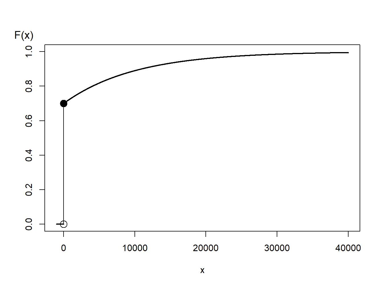
Figure 6.3: Distribution Function of a Hybrid Random Variable
From Figure 6.3, we can see that the inverse transform for generating random variables with this distribution function is
\[ \begin{aligned} X = F^{-1}(U) = \left\{ \begin{array}{cc} 0 & 0< U \leq 0.7 \\ -1000 \ln (\frac{1-U}{0.3}) & 0.7 < U < 1 . \end{array} \right. \end{aligned} \]
For discrete and hybrid random variables, the key is to draw a graph of the distribution function that allows you to visualize potential values of the inverse function.
6.1.3 Simulation Precision
From the prior subsections, we now know how to generate independent simulated realizations from a distribution of interest. With these realizations, we can construct an empirical distribution and approximate the underlying distribution as precisely as needed. As we introduce more actuarial applications in this book, you will see that simulation can be applied in a wide variety of contexts.
Many of these applications can be reduced to the problem of approximating \(\mathrm{E~}[h(X)]\), where \(h(\cdot)\) is some known function. Based on \(R\) simulations (replications), we get \(X_1,\ldots,X_R\). From this simulated sample, we calculate an average
\[ \overline{h}_R=\frac{1}{R}\sum_{i=1}^{R} h(X_i) \] that we use as our simulated approximate (estimate) of \(\mathrm{E~}[h(X)]\). To estimate the precision of this approximation, we use the simulation variance
\[ s_{h,R}^2 = \frac{1}{R-1} \sum_{i=1}^{R}\left( h(X_i) -\overline{h}_R \right) ^2. \]
From the independence, the standard error of the estimate is \(s_{h,R}/\sqrt{R}\). This can be made as small as we like by increasing the number of replications \(R\).
Example 6.1.8. Portfolio Management. In Section 3.4, we learned how to calculate the expected value of policies with deductibles. For an example of something that cannot be done with closed form expressions, we now consider two risks. This is a variation of a more complex example that will be covered as Example 10.3.6.
We consider two property risks of a telecommunications firm:
- \(X_1\) - buildings, modeled using a gamma distribution with mean 200 and scale parameter 100.
- \(X_2\) - motor vehicles, modeled using a gamma distribution with mean 400 and scale parameter 200.
Denote the total risk as \(X = X_1 + X_2.\) For simplicity, you assume that these risks are independent.
To manage the risk, you seek some insurance protection. You are willing to retain internally small building and motor vehicles amounts, up to \(M\), say. Random amounts in excess of \(M\) will have an unpredictable affect on your budget and so for these amounts you seek insurance protection. Stated mathematically, your retained risk is \(Y_{retained}=\) \(\min(X_1 + X_2,M)\) and the insurer’s portion is \(Y_{insurer} = X- Y_{retained}\).
To be specific, we use \(M=\) 400 as well as \(R=\) 1000000 simulations.
a. With the settings, we wish to determine the expected claim amount and the associated standard deviation of (i) that retained, (ii) that accepted by the insurer, and (iii) the total overall amount.
Show R Code to Define the Risks
Here is the code for the expected claim amounts.
Show R Code To Compute Amounts
The results of these calculations are:
                   Retained Insurer  Total
Mean                 365.17  235.01 600.18
Standard Deviation 69.51 280.86 316.36b. For insured claims, the standard error of the simulation approximation is \(s_{h,R}/\sqrt{1000000} =\) 280.86 \(/\sqrt{1000000} =\) 0.281. For this example, simulation is quick and so a large value such as 1000000 is an easy choice. However, for more complex problems, the simulation size may be an issue.
Show R Code To Set up the Visualization
Figure 6.4 allows us to visualize the development of the approximation as the number of simulations increases.
matplot(1:R,sumP2[,1:20],type="l",col=rgb(1,0,0,.2), ylim=c(100, 400),
        xlab=expression(paste("Number of Simulations (", italic('R'), ")")),
        ylab="Expected Insurer Claims")
abline(h=mean(Yinsurer),lty=2)
bonds <- cbind(1.96*sd(Yinsurer)*sqrt(1/(1:R)),-1.96*sd(Yinsurer)*sqrt(1/(1:R)))
matlines(1:R,bonds+mean(Yinsurer),col="red",lty=1)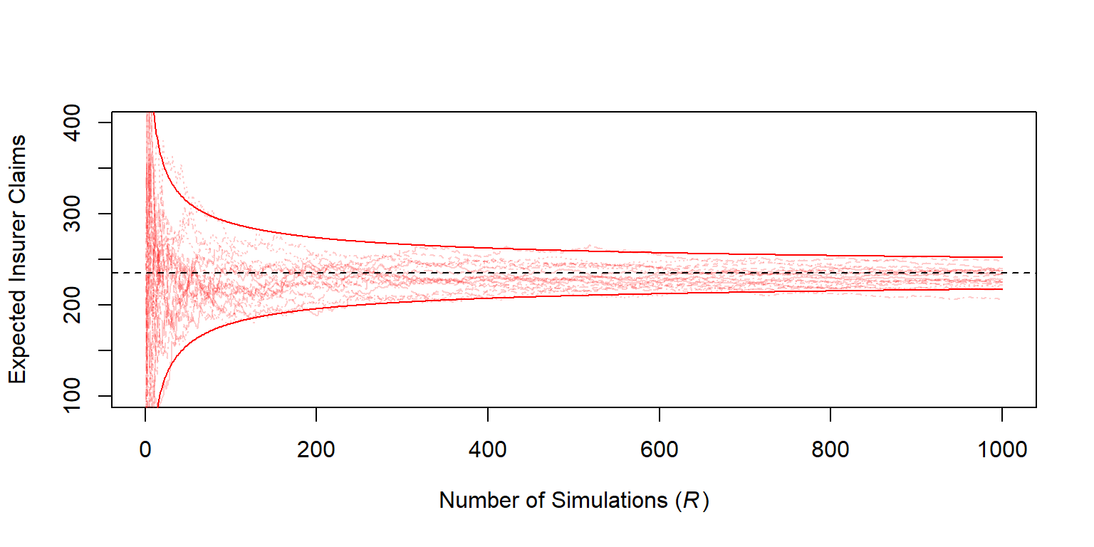
Figure 6.4: Estimated Expected Insurer Claims versus Number of Simulations
Determination of Number of Simulations
How many simulated values are recommended? 100? 1,000,000? We can use the central limit theoremThe sample mean and sample sum of a random sample of n from a population will converge to a normal curve as the sample size n grows to respond to this question.
As one criterion for your confidence in the result, suppose that you wish to be within 1% of the mean with 95% certainty. That is, you want \(\Pr \left( |\overline{h}_R - \mathrm{E~}[h(X)]| \le 0.01 \mathrm{E~}[h(X)] \right) \ge 0.95\). According to the central limit theorem, your estimate should be approximately normally distributed and so we want to have \(R\) large enough to satisfy \(0.01 \mathrm{E~}[h(X)]/\sqrt{\mathrm{Var~}[h(X)]/R}) \ge 1.96\). (Recall that 1.96 is the 97.5th percentile from the standard normal distribution.) Replacing \(\mathrm{E~}[h(X)]\) and \(\mathrm{Var~}[h(X)]\) with estimates, you continue your simulation until
\[ \frac{.01\overline{h}_R}{s_{h,R}/\sqrt{R}}\geq 1.96 \] or equivalently
\[\begin{equation} R \geq 38,416\frac{s_{h,R}^2}{\overline{h}_R^2}. \tag{6.1} \end{equation}\]
This criterion is a direct application of the approximate normality. Note that \(\overline{h}_R\) and \(s_{h,R}\) are not known in advance, so you will have to come up with estimates, either by doing a small pilot study in advance or by interrupting your procedure intermittently to see if the criterion is satisfied.
Example 6.1.8. Portfolio Management - continued
For our example, the average insurance claim is 235.011 and the corresponding standard deviation is 280.862. Using equation (6.1), to be within 10% of the mean, we would only require at least 54.87 thousand simulations. However, to be within 1% we would want at least 5.49 million simulations.
Example 6.1.9. Approximation Choices. An important application of simulation is the approximation of \(\mathrm{E~}[h(X)]\). In this example, we show that the choice of the \(h(\cdot)\) function and the distribution of \(X\) can play a role.
Consider the following question : what is \(\Pr[X>2]\) when \(X\) has a Cauchy distributionA continuous distribution that represents the distribution of the ratio of two independent normally random variables, where the denominator distribution has mean zero, with density \(f(x) =\left(\pi(1+x^2)\right)^{-1}\), on the real line? The true value is
\[
\Pr\left[X>2\right] = \int_2^\infty \frac{dx}{\pi(1+x^2)} .
\]
One can use an R numerical integration function (which usually works well on improper integrals)
which is equal to 0.14758.
Approximation 1. Alternatively, one can use simulation techniques to approximate that quantity. From calculus, you can check that the quantile function of the Cauchy distribution is \(F^{-1}(y) = \tan \left( \pi(y-0.5) \right)\). Then, with simulated uniform (0,1) variates, \(U_1, \ldots, U_R\), we can construct the estimator
\[ p_1 = \frac{1}{R}\sum_{i=1}^R \mathrm{I}(F^{-1}(U_i)>2) = \frac{1}{R}\sum_{i=1}^R \mathrm{I}(\tan \left( \pi(U_i-0.5) \right)>2) . \]
Show the R Code
With one million simulations, we obtain an estimate of 0.14744 with standard error 0.355 (divided by 1000). One can prove that the variance of \(p_1\) is of order \(0.127/R\).
Approximation 2. With other choices of \(h(\cdot)\) and \(F(\cdot)\) it is possible to reduce uncertainty even using the same number of simulations \(R\). To begin, one can use the symmetry of the Cauchy distribution to write \(\Pr[X>2]=0.5\cdot\Pr[|X|>2]\). With this, can construct a new estimator,
\[ p_2 = \frac{1}{2R}\sum_{i=1}^R \mathrm{I}(|F^{-1}(U_i)|>2) . \]
With one million simulations, we obtain an estimate of 0.14748 with standard error 0.228 (divided by 1000). One can prove that the variance of \(p_2\) is of order \(0.052/R\).
Approximation 3. But one can go one step further. The improper integral can be written as a proper one by a simple symmetry property (since the function is symmetric and the integral on the real line is equal to \(1\)) \[ \int_2^\infty \frac{dx}{\pi(1+x^2)}=\frac{1}{2}-\int_0^2\frac{dx}{\pi(1+x^2)} . \] From this expression, a natural approximation would be \[ p_3 = \frac{1}{2}-\frac{1}{R}\sum_{i=1}^R h_3(2U_i), ~~~~~~\text{where}~h_3(x)=\frac{2}{\pi(1+x^2)} . \]
With one million simulations, we obtain an estimate of 0.14756 with standard error 0.169 (divided by 1000). One can prove that the variance of \(p_3\) is of order \(0.0285/R\).
Approximation 4. Finally, one can also consider some change of variable in the integral \[ \int_2^\infty \frac{dx}{\pi(1+x^2)}=\int_0^{1/2}\frac{y^{-2}dy}{\pi(1-y^{-2})} . \] From this expression, a natural approximation would be \[ p_4 = \frac{1}{R}\sum_{i=1}^R h_4(U_i/2),~~~~~\text{where}~h_4(x)=\frac{1}{2\pi(1+x^2)} . \] The expression seems rather similar to the previous one.
With one million simulations, we obtain an estimate of 0.14759 with standard error 0.01 (divided by 1000). One can prove that the variance of \(p_4\) is of order \(0.00009/R\), which is much smaller than what we had so far!
Table 6.1 summarizes the four choices of \(h(\cdot)\) and \(F(\cdot)\) to approximate \(\Pr[X>2] =\) 0.14758. The standard error varies dramatically. Thus, if we have a desired degree of accuracy, then the number of simulations depends strongly on how we write the integrals we try to approximate.
Table 6.1. Summary of Four Choices to Approximate \(\Pr[X>2]\)
| Estimator | Definition | Support Function | Estimate | Standard Error |
|---|---|---|---|---|
| \(p_1\) | \(\frac{1}{R}\sum_{i=1}^R \mathrm{I}(F^{-1}(U_i)>2)\) | \(~~~~~~F^{-1}(u)=\tan \left( \pi(u-0.5) \right)~~~~~~~\) | 0.147439 | 0.000355 |
| \(p_2\) | \(\frac{1}{2R}\sum_{i=1}^R \mathrm{I}(|F^{-1}(U_i)|>2)\) | \(F^{-1}(u)=\tan \left( \pi(u-0.5) \right)\) | 0.147477 | 0.000228 |
| \(p_3\) | \(\frac{1}{2}-\frac{1}{R}\sum_{i=1}^R h_3(2U_i)\) | \(h_3(x)=\frac{2}{\pi(1+x^2)}\) | 0.147558 | 0.000169 |
| \(p_4\) | \(\frac{1}{R}\sum_{i=1}^R h_4(U_i/2)\) | \(h_4(x)=\frac{1}{2\pi(1+x^2)}\) | 0.147587 | 0.000010 |
6.1.4 Simulation and Statistical Inference
Simulations not only help us approximate expected values but are also useful in calculating other aspects of distribution functions. In particular, they are very useful when distributions of test statistics are too complicated to derive; in this case, one can use simulations to approximate the reference distribution. We now illustrate this with the Kolmogorov-Smirnov testA nonparametric statistical test used to determine if a data sample could come from a hypothesized continuous probability distribution that we learned about in Section 4.1.2.2.
Example 6.1.10. Kolmogorov-Smirnov Test of Distribution. Suppose that we have available \(n=100\) observations \(\{x_1,\cdots,x_n\}\) that, unknown to the analyst, were generated from a gamma distribution with parameters \(\alpha = 6\) and \(\theta=2\). The analyst believes that the data come from a lognormal distribution with parameters 1 and 0.4 and would like to test this assumption.
The first step is to visualize the data.
Show R Code To Set up The Visualization
With this set-up, Figure 6.5 provides a graph of a histogram and empirical distribution. For reference, superimposed are red dashed lines from the lognormal distribution.
par(mfrow=c(1,2))
hist(x,probability = TRUE,main="Histogram", col="light blue",
     border="white",xlim=c(0,7),ylim=c(0,.4))
lines(u,dlnorm(u,1,.4),col="red",lty=2)
plot(vx,vy,type="l",xlab="x",ylab="Cumulative Distribution",main="Empirical cdf")
lines(u,plnorm(u,1,.4),col="red",lty=2)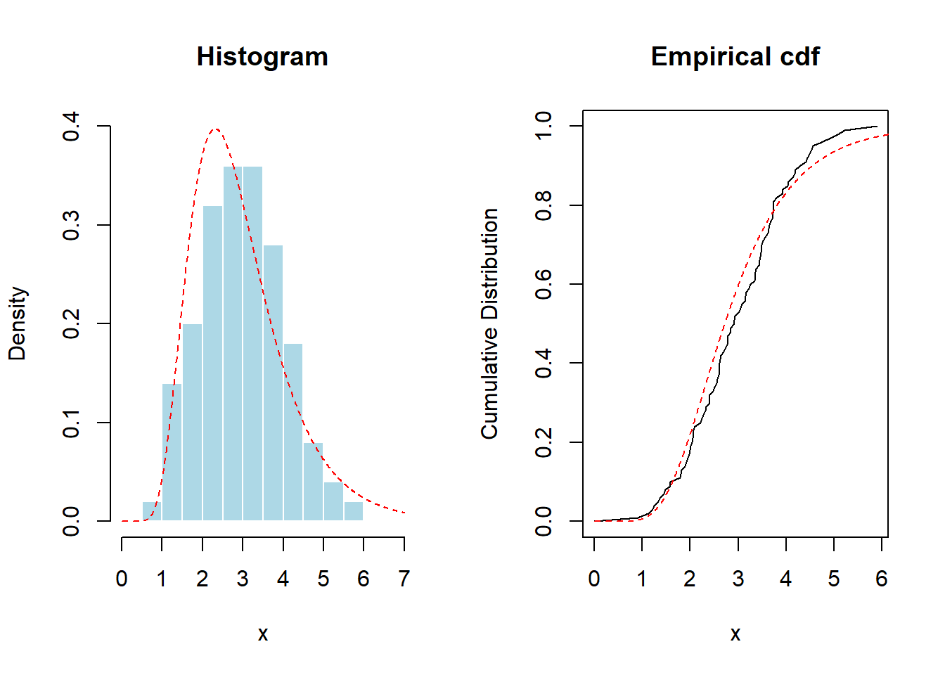
Figure 6.5: Histogram and Empirical Distribution Function of Data used in Kolmogorov-Smirnov Test. The red dashed lines are fits based on (incorrectly) hypothesized lognormal distribution.
Recall that the Kolmogorov-Smirnov statistic equals the largest discrepancy between the empirical and the hypothesized distribution. This is \(\max_x |F_n(x)-F_0(x)|\), where \(F_0\) is the hypothesized lognormal distribution. We can calculate this directly as:
Show R Code for a Direct Calculation of the KS Statistic
Fortunately, for the lognormal distribution, R has built-in tests that allow us to determine this without complex programming:
    One-sample Kolmogorov-Smirnov test

data:  x
D = 0.097037, p-value = 0.3031
alternative hypothesis: two-sided
However, for many distributions of actuarial interest, pre-built programs are not available. We can use simulation to test the relevance of the test statistic. Specifically, to compute the \(p\)-value, let us generate thousands of random samples from a \(LN(1,0.4)\) distribution (with the same size), and compute empirically the distribution of the statistic,
Show R Code for the Simulation Distribution of the KS Statistic
hist(d_KS,probability = TRUE,col="light blue",border="white",xlab="Test Statistic",main="")
lines(density(d_KS),col="red")
abline(v=D(x,function(x) plnorm(x,1,.4)),lty=2,col="red")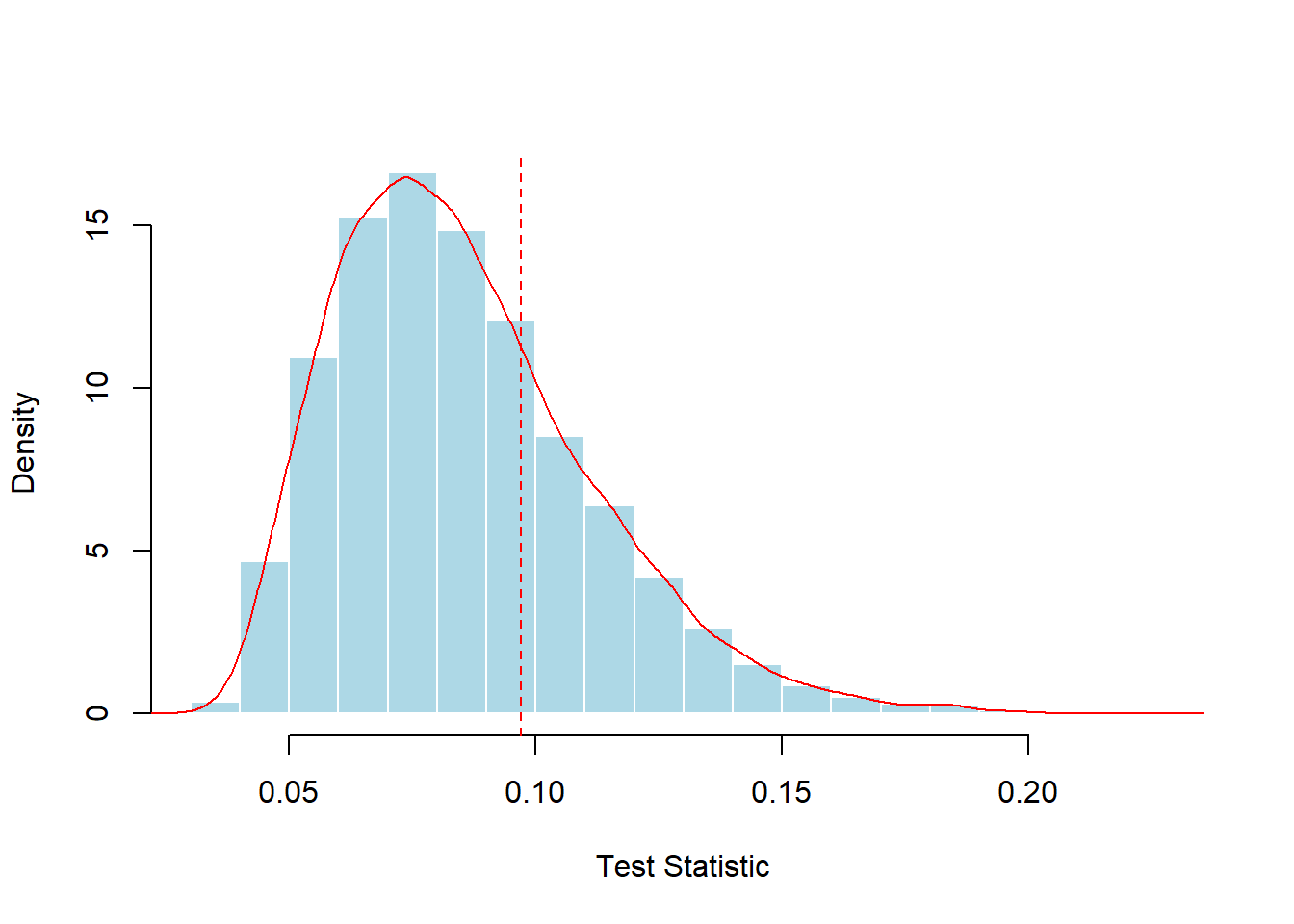
Figure 6.6: Simulated Distribution of the Kolmogorov-Smirnov Test Statistic. The vertical red dashed line marks the test statistic for the sample of 100.
The simulated distribution based on 10,000 random samples is summarized in Figure 6.6. Here, the statistic exceeded the empirical value (0.09704) in 28.43% of the scenarios, while the theoretical \(p\)-value is 0.3031. For both the simulation and the theoretical \(p\)-values, the conclusions are the same; the data do not provide sufficient evidence to reject the hypothesis of a lognormal distribution.
Although only an approximation, the simulation approach works in a variety of distributions and test statistics without needing to develop the nuances of the underpinning theory for each situation. We summarize the procedure for developing simulated distributions and p-values as follows:
- Draw a sample of size n, say, \(X_1, \ldots, X_n\), from a known distribution function \(F\). Compute a statistic of interest, denoted as \(\hat{\theta}(X_1, \ldots, X_n)\). Call this \(\hat{\theta}^r\) for the rth replication.
- Repeat this \(r=1, \ldots, R\) times to get a sample of statistics, \(\hat{\theta}^1, \ldots,\hat{\theta}^R\).
- From the sample of statistics in Step 2, \(\{\hat{\theta}^1, \ldots,\hat{\theta}^R\}\), compute a summary measure of interest, such as a p-value.
6.2 Bootstrapping and Resampling
In this section, you learn how to:
- Generate a nonparametric bootstrap distribution for a statistic of interest
- Use the bootstrap distribution to generate estimates of precision for the statistic of interest, including bias, standard deviations, and confidence intervals
- Perform bootstrap analyses for parametric distributions
6.2.1 Bootstrap Foundations
Simulation presented up to now is based on sampling from a known distribution. Section 6.1 showed how to use simulation techniques to sample and compute quantities from known distributions. However, statistical science is dedicated to providing inferences about distributions that are unknown. We gather summary statistics based on this unknown population distribution. But how do we sample from an unknown distribution?
Naturally, we cannot simulate draws from an unknown distribution but we can draw from a sample of observations. If the sample is a good representation from the population, then our simulated draws from the sample should well approximate the simulated draws from a population. The process of sampling from a sample is called resampling or bootstrapping. The term bootstrapA method of sampling with replacement from the original dataset to create additional simulated datasets of the same size as the original comes from the phrase “pulling oneself up by one’s bootstraps” (Efron, 1979). With resampling, the original sample plays the role of the population and estimates from the sample play the role of true population parameters.
The resampling algorithm is the same as introduced in Section 6.1.4 except that now we use simulated draws from a sample. It is common to use \(\{X_1, \ldots, X_n\}\) to denote the original sample and let \(\{X_1^*, \ldots, X_n^*\}\) denote the simulated draws. We draw them with replacement so that the simulated draws will be independent from one another, the same assumption as with the original sample. For each sample, we also use n simulated draws, the same number as the original sample size. To distinguish this procedure from the simulation, it is common to use B (for bootstrap) to be the number of simulated samples. We could also write \(\{X_1^{(b)}, \ldots, X_n^{(b)}\}\), \(b=1,\ldots, B\) to clarify this.
There are two basic resampling methods, model-free and model-based, which are, respectively, as nonparametric and parametric. In the nonparametric approachA statistical method where no assumption is made about the distribution of the population, no assumption is made about the distribution of the parent population. The simulated draws come from the empirical distribution function \(F_n(\cdot)\), so each draw comes from \(\{X_1, \ldots, X_n\}\) with probability 1/n.
In contrast, for the parametric approachA statistical method where a prior assumption is made about the distribution or model form, we assume that we have knowledge of the distribution family F. The original sample \(X_1, \ldots, X_n\) is used to estimate parameters of that family, say, \(\hat{\theta}\). Then, simulated draws are taken from the \(F(\hat{\theta})\). Section 6.2.4 discusses this approach in further detail.
Nonparametric Bootstrap
The idea of the nonparametric bootstrap is to use the inverse transform method on \(F_n\), the empirical cumulative distribution function, depicted in Figure 6.7.
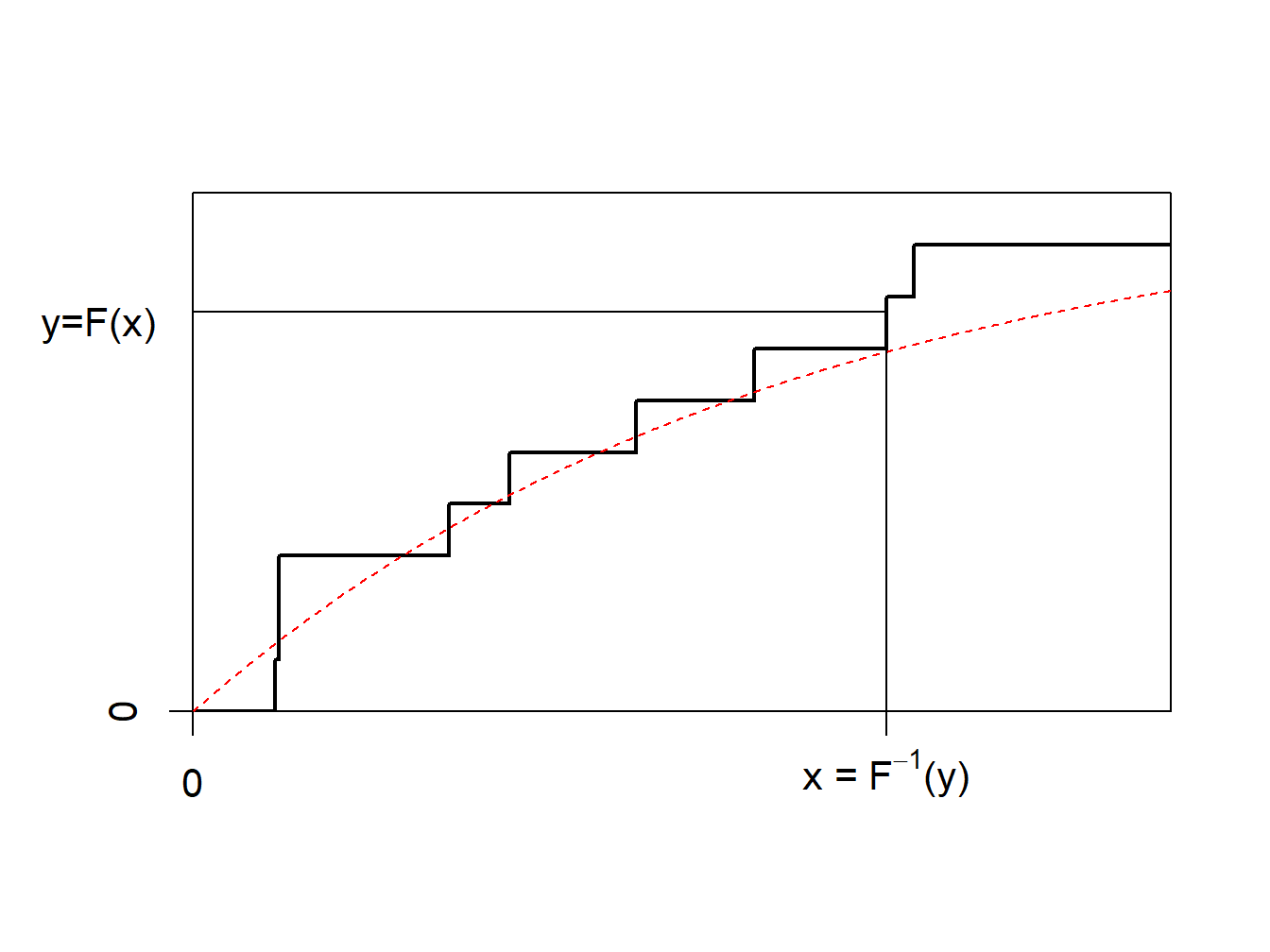
Figure 6.7: Inverse of an Empirical Distribution Function
Because \(F_n\) is a step-function, \(F_n^{-1}\) takes values in \(\{x_1,\cdots,x_n\}\). More precisely, as illustrated in Figure 6.8.
- if \(y\in(0,1/n)\) (with probability \(1/n\)) we draw the smallest value (\(\min\{x_i\}\))
- if \(y\in(1/n,2/n)\) (with probability \(1/n\)) we draw the second smallest value,
- …
- if \(y\in((n-1)/n,1)\) (with probability \(1/n\)) we draw the largest value (\(\max\{x_i\}\)).
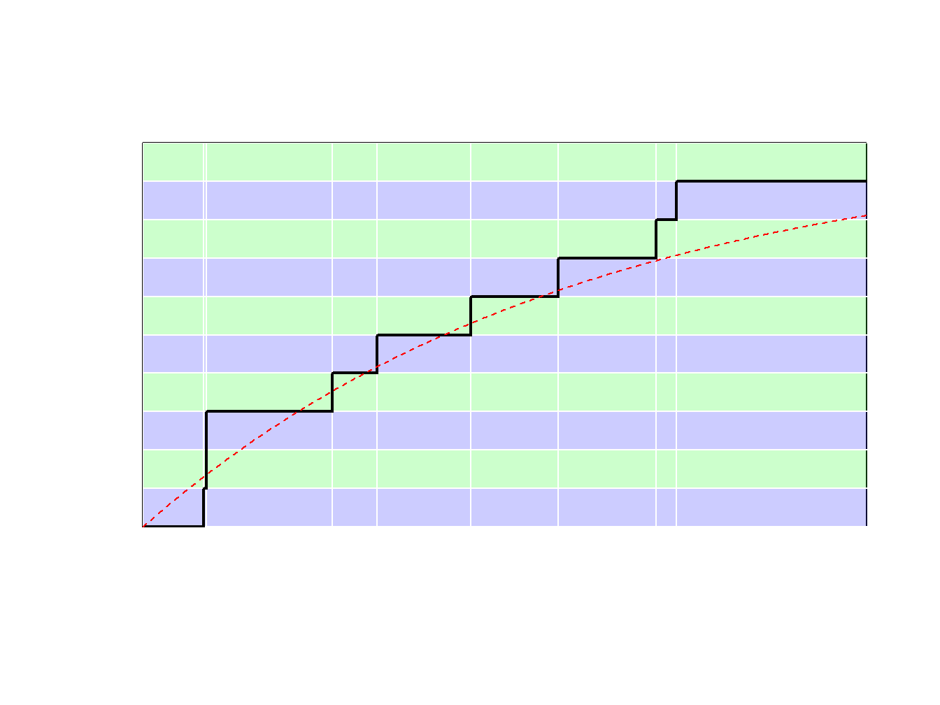
Figure 6.8: Inverse of an Empirical Distribution Function
Using the inverse transform method with \(F_n\) means sampling from \(\{x_1,\cdots,x_n\}\), with probability \(1/n\). Generating a bootstrap sample of size \(B\) means sampling from \(\{x_1,\cdots,x_n\}\), with probability \(1/n\), with replacement. See the following illustrative R code.
Show R Code For Creating a Bootstrap Sample
[1] 2.6164 5.7394 5.7394 2.6164 2.6164 7.0899 0.8823 5.7394Observe that value 0.8388 was obtained three times.
6.2.2 Bootstrap Precision: Bias, Standard Deviation, and Mean Square Error
We summarize the nonparametric bootstrap procedure as follows:
- From the sample \(\{X_1, \ldots, X_n\}\), draw a sample of size n (with replacement), say, \(X_1^*, \ldots, X_n^*\). From the simulated draws compute a statistic of interest, denoted as \(\hat{\theta}(X_1^*, \ldots, X_n^*)\). Call this \(\hat{\theta}_b^*\) for the bth replicate.
- Repeat this \(b=1, \ldots, B\) times to get a sample of statistics, \(\hat{\theta}_1^*, \ldots,\hat{\theta}_B^*\).
- From the sample of statistics in Step 2, \(\{\hat{\theta}_1^*, \ldots, \hat{\theta}_B^*\}\), compute a summary measure of interest.
In this section, we focus on three summary measures, the biasThe difference between the expected value of an estimator and the parameter being estimated. bias is an estimation error that does not become smaller as one observes larger sample sizes., the standard deviation, and the mean square error (MSE). Table 6.2 summarizes these three measures. Here, \(\overline{\hat{\theta^*}}\) is the average of \(\{\hat{\theta}_1^*, \ldots,\hat{\theta}_B^*\}\).
Table 6.2. Bootstrap Summary Measures
\[ {\small \begin{matrix} \begin{array}{l|c|c|c} \hline \text{Population Measure}& \text{Population Definition}&\text{Bootstrap Approximation}&\text{Bootstrap Symbol}\\ \hline \text{Bias} & \mathrm{E}(\hat{\theta})-\theta&\overline{\hat{\theta^*}}-\hat{\theta}& Bias_{boot}(\hat{\theta}) \\\hline \text{Standard Deviation} & \sqrt{\mathrm{Var}(\hat{\theta})} & \sqrt{\frac{1}{B-1} \sum_{b=1}^{B}\left(\hat{\theta}_b^* -\overline{\hat{\theta^*}} \right) ^2}&s_{boot}(\hat{\theta}) \\\hline \text{Mean Square Error} &\mathrm{E}(\hat{\theta}-\theta)^2 & \frac{1}{B} \sum_{b=1}^{B}\left(\hat{\theta}_b^* -\hat{\theta} \right)^2&MSE_{boot}(\hat{\theta})\\ \hline \end{array}\end{matrix} } \]
Example 6.2.1. Bodily Injury Claims and Loss Elimination Ratios. To show how the bootstrap can be used to quantify the precision of estimators, we return to the Section 4.1.1.5 Example 4.1.6 bodily injury claims data where we introduced a nonparametric estimator of the loss elimination ratio.
Table 6.3 summarizes the results of the bootstrap estimation. For example, at \(d=14000\), the nonparametric estimate of LER is 0.97678. This has an estimated bias of 0.00018 with a standard deviation of 0.00701. For some applications, you may wish to apply the estimated bias to the original estimate to give a bias-corrected estimatorIf an estimator is known to be consistently biased in a manner, it can be corrected using a factor to be come less biased or unbiased. This is the focus of the next example. For this illustration, the bias is small and so such a correction is not relevant.
Show R Code For Bootstrap Estimates of LER
Table 6.3. Bootstrap Estimates of LER at Selected Deductibles
| d | NP Estimate | Bootstrap Bias | Bootstrap SD | Lower Normal 95% CI | Upper Normal 95% CI |
|---|---|---|---|---|---|
| 4000 | 0.54113 | 0.00011 | 0.01237 | 0.51678 | 0.56527 |
| 5000 | 0.64960 | 0.00027 | 0.01412 | 0.62166 | 0.67700 |
| 10500 | 0.93563 | 0.00004 | 0.01017 | 0.91567 | 0.95553 |
| 11500 | 0.95281 | -0.00003 | 0.00941 | 0.93439 | 0.97128 |
| 14000 | 0.97678 | 0.00016 | 0.00687 | 0.96316 | 0.99008 |
| 18500 | 0.99382 | 0.00014 | 0.00331 | 0.98719 | 1.00017 |
The bootstrap standard deviation gives a measure of precision. For one application of standard deviations, we can use the normal approximation to create a confidence interval. For example, the R function boot.ci produces the normal confidence intervals at 95%. These are produced by creating an interval of twice the length of 1.95994 bootstrap standard deviations, centered about the bias-corrected estimator (1.95994 is the 97.5th quantile of the standard normal distribution). For example, the lower normal 95% CI at \(d=14000\) is \((0.97678-0.00018)- 1.95994*0.00701\) \(= 0.96286\). We further discuss bootstrap confidence intervals in the next section.
Example 6.2.2. Estimating \(\exp(\mu)\). The bootstrap can be used to quantify the bias of an estimator, for instance. Consider here a sample \(\mathbf{x}=\{x_1,\cdots,x_n\}\) that is iidIndependent and identically distributed with mean \(\mu\).
sample_x <- c(2.46,2.80,3.28,3.86,2.85,3.67,3.37,3.40,5.22,2.55,
              2.79,4.50,3.37,2.88,1.44,2.56,2.00,2.07,2.19,1.77)
Suppose that the quantity of interest is \(\theta=\exp(\mu)\). A natural estimator would be \(\widehat{\theta}_1=\exp(\overline{x})\). This estimator is biased (due to the Jensen inequalityFor a convex function f(x), f(expected value of x) <= expected value of f(x)) but is asymptotically unbiased. For our sample, the estimate is as follows.
[1] 19.13463One can use the central limit theorem to get a correction using \[ \overline{X}\approx\mathcal{N}\left(\mu,\frac{\sigma^2}{n}\right)\text{ where }\sigma^2=\text{Var}[X_i] , \] so that, with the normal moment generating function, we have \[ \mathrm{E}~\left[\exp(\overline{X})\right] \approx \exp\left(\mu+\frac{\sigma^2}{2n}\right) . \] Hence, one can consider naturally \[ \widehat{\theta}_2=\exp\left(\overline{x}-\frac{\widehat{\sigma}^2}{2n}\right) . \] For our data, this turns out to be as follows.
[1] 18.73334As another strategy (that we do not pursue here), one can also use Taylor’s approximation to get a more accurate estimator (as in the delta method), \[ g(\overline{x})=g(\mu)+(\overline{x}-\mu)g'(\mu)+(\overline{x}-\mu)^2\frac{g''(\mu)}{2}+\cdots \] The alternative we do explore is to use a bootstrap strategy: given a bootstrap sample, \(\mathbf{x}^{\ast}_{b}\), let \(\overline{x}^{\ast}_{b}\) denote its mean, and set
\[ \widehat{\theta}_3=\frac{1}{B}\sum_{b=1}^B\exp(\overline{x}^{\ast}_{b}) . \] To implement this, we have the following code.
Show R Code for Creating Bootstrap Samples
Then, you can plot(results) and print(results) to see the following.
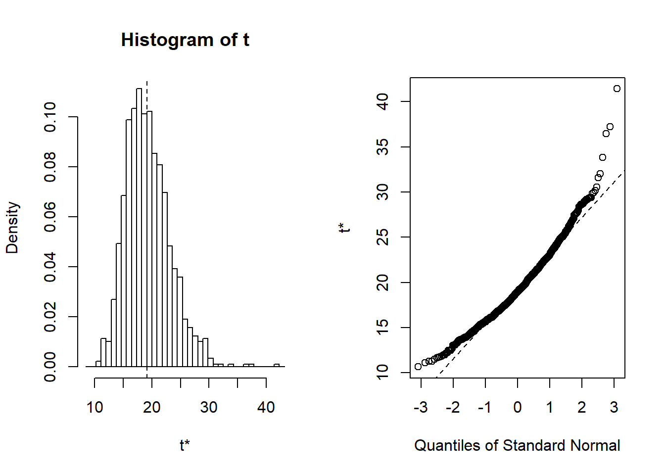
Figure 6.9: Distribution of Bootstrap Replicates. The left-hand panel is a histogram of replicates. The right-hand panel is a quantile-quantile plot, comparing the bootstrap distribution to the standard normal distribution.
ORDINARY NONPARAMETRIC BOOTSTRAP


Call:
boot(data = sample_x, statistic = function(y, indices) exp(mean(y[indices])),
    R = 1000)


Bootstrap Statistics :
    original    bias    std. error
t1* 19.13463 0.2536551    3.909725
This results in three estimators, the raw estimator \(\widehat{\theta}_1=\) 19.135, the second-order correction \(\widehat{\theta}_2=\) 18.733, and the bootstrap estimator \(\widehat{\theta}_3=\) 19.388.
How does this work with differing sample sizes? We now suppose that the \(x_i\)’s are generated from a lognormal distribution \(LN(0,1)\), so that \(\mu = \exp(0 + 1/2) = 1.648721\) and \(\theta = \exp(1.648721)\) \(= 5.200326\). We use simulation to draw the sample sizes but then act as if they were a realized set of observations. See the following illustrative code.
Show R Code for Creating Bootstrap Samples
The results of the comparison are summarized in Figure 6.10. This figure shows that the bootstrap estimator is closer to the true parameter value for almost all sample sizes. The bias of all three estimators decreases as the sample size increases.
matplot(VN,t(Est),type="l", col=2:4, lty=2:4, ylim=exp(exp(1/2))+c(-1,1),
        xlab="sample size (n)", ylab="estimator")
abline(h=exp(exp(1/2)),lty=1, col=1)
legend("topleft", c("raw estimator", "second order correction", "bootstrap"),
       col=2:4,lty=2:4, bty="n")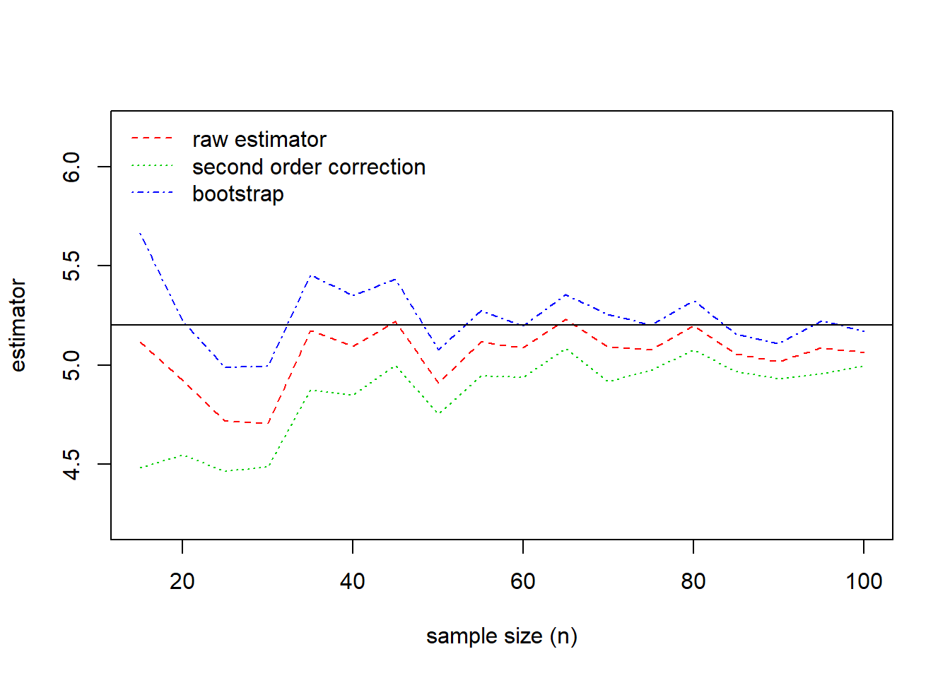
Figure 6.10: Comparision of Estimates. True value of the parameter is given by the solid horizontal line at 5.20.
6.2.3 Confidence Intervals
The bootstrap procedure generates B replicates \(\hat{\theta}_1^*, \ldots,\hat{\theta}_B^*\) of the estimator \(\hat{\theta}\). In Example 6.2.1, we saw how to use standard normal approximations to create a confidence interval for parameters of interest. However, given that a major point is to use bootstrapping to avoid relying on assumptions of approximate normality, it is not surprising that there are alternative confidence intervals available.
For an estimator \(\hat{\theta}\), the basic bootstrap confidence interval is
\[\begin{equation} \left(2 \hat{\theta} - q_U, 2 \hat{\theta} - q_L \right) , \tag{6.2} \end{equation}\]
where \(q_L\) and \(q_U\) are lower and upper 2.5% quantiles from the bootstrap sample \(\hat{\theta}_1^*, \ldots,\hat{\theta}_B^*\).
To see where this comes from, start with the idea that \((q_L, q_U)\) provides a 95% interval for \(\hat{\theta}_1^*, \ldots,\hat{\theta}_B^*\). So, for a random \(\hat{\theta}_b^*\), there is a 95% chance that \(q_L \le \hat{\theta}_b^* \le q_U\). Reversing the inequalities and adding \(\hat{\theta}\) to each side gives a 95% interval
\[ \hat{\theta} -q_U \le \hat{\theta} - \hat{\theta}_b^* \le \hat{\theta} -q_L . \] So, \(\left( \hat{\theta}-q_U, \hat{\theta} -q_L\right)\) is an 95% interval for \(\hat{\theta} - \hat{\theta}_b^*\). The bootstrap approximation idea says that this is also a 95% interval for \(\theta - \hat{\theta}\). Adding \(\hat{\theta}\) to each side gives the 95% interval in equation (6.2).
Many alternative bootstrap intervals are available. The easiest to explain is the percentile bootstrap intervalConfidence interval for the parameter estimates determined using the actual percentile results from the bootstrap sampling approach, as every bootstrap sample has an associated parameter estimate(s) that can be ranked against the others which is defined as \(\left(q_L, q_U\right)\). However, this has the drawback of potentially poor behavior in the tails which can be of concern in some actuarial problems of interest.
Example 6.2.3. Bodily Injury Claims and Risk Measures. To see how the bootstrap confidence intervals work, we return to the bodily injury auto claims considered in Example 6.2.1. Instead of the loss elimination ratio, suppose we wish to estimate the 95th percentile \(F^{-1}(0.95)\) and a measure defined as \[ TVaR_{0.95}[X] = \mathrm{E}[X | X > F^{-1}(0.95)] . \] This measure is called the tail value-at-riskThe expected value of a risk given that the risk exceeds a value-at-risk; it is the expected value of \(X\) conditional on \(X\) exceeding the 95th percentile. Section 10.2 explains how quantiles and the tail value-at-risk are the two most important examples of so-called risk measures. For now, we will simply think of these as measures that we wish to estimate. For the percentile, we use the nonparametric estimator \(F^{-1}_n(0.95)\) defined in Section 4.1.1.3. For the tail value-at-risk, we use the plug-in principle to define the nonparametric estimator
\[ TVaR_{n,0.95}[X] = \frac{\sum_{i=1}^n X_i I(X_i > F^{-1}_n(0.95))}{\sum_{i=1}^n I(X_i > F^{-1}_n(0.95))} ~. \] In this expression, the denominator counts the number of observations that exceed the 95th percentile \(F^{-1}_n(0.95)\). The numerator adds up losses for those observations that exceed \(F^{-1}_n(0.95)\). Table 6.4 summarizes the estimator for selected fractions.
Show R Code for Creating Quantile Bootstrap Samples
Table 6.4. Bootstrap Estimates of Quantiles at Selected Fractions
| Fraction | NP Estimate | Bootstrap Bias | Bootstrap SD | Lower Normal 95% CI | Upper Normal 95% CI | Lower Basic 95% CI | Upper Basic 95% CI | Lower Percentile 95% CI | Upper Percentile 95% CI |
|---|---|---|---|---|---|---|---|---|---|
| 0.50 | 6500.00 | -128.02 | 200.36 | 6235.32 | 7020.72 | 6300.00 | 7000.00 | 6000.00 | 6700.00 |
| 0.80 | 9078.40 | 89.51 | 200.27 | 8596.38 | 9381.41 | 8533.20 | 9230.40 | 8926.40 | 9623.60 |
| 0.90 | 11454.00 | 55.95 | 480.66 | 10455.96 | 12340.13 | 10530.49 | 12415.00 | 10493.00 | 12377.51 |
| 0.95 | 13313.40 | 13.59 | 667.74 | 11991.07 | 14608.55 | 11509.70 | 14321.00 | 12305.80 | 15117.10 |
| 0.98 | 16758.72 | 101.46 | 1273.45 | 14161.34 | 19153.19 | 14517.44 | 19326.95 | 14190.49 | 19000.00 |
For example, when the fraction is 0.50, we see that lower and upper 2.5th quantiles of the bootstrap simulations are \(q_L=\) 6000 and \(q_u=\) 6700, respectively. These form the percentile bootstrap confidence interval. With the nonparametric estimator 6500, these yield the lower and upper bounds of the basic confidence interval 6300 and 7000, respectively. Table 6.4 also shows bootstrap estimates of the bias, standard deviation, and a normal confidence interval, concepts introduced in Section 6.2.2.
Table 6.5 shows similar calculations for the tail value-at-risk. In each case, we see that the bootstrap standard deviation increases as the fraction increases. This is because there are fewer observations to estimate quantiles as the fraction increases, leading to greater imprecision. Confidence intervals also become wider. Interestingly, there does not seem to be the same pattern in the estimates of the bias.
Show R Code for Creating TVar Bootstrap Samples
Table 6.5. Bootstrap Estimates of TVaR at Selected Risk Levels
| Fraction | NP Estimate | Bootstrap Bias | Bootstrap SD | Lower Normal 95% CI | Upper Normal 95% CI | Lower Basic 95% CI | Upper Basic 95% CI | Lower Percentile 95% CI | Upper Percentile 95% CI |
|---|---|---|---|---|---|---|---|---|---|
| 0.50 | 9794.69 | -120.82 | 273.35 | 9379.74 | 10451.27 | 9355.14 | 10448.87 | 9140.51 | 10234.24 |
| 0.80 | 12454.18 | 30.68 | 481.88 | 11479.03 | 13367.96 | 11490.62 | 13378.52 | 11529.84 | 13417.74 |
| 0.90 | 14720.05 | 17.51 | 718.23 | 13294.82 | 16110.25 | 13255.45 | 16040.72 | 13399.38 | 16184.65 |
| 0.95 | 17072.43 | 5.99 | 1103.14 | 14904.31 | 19228.56 | 14924.50 | 19100.88 | 15043.97 | 19220.36 |
| 0.98 | 20140.56 | 73.43 | 1587.64 | 16955.40 | 23178.85 | 16942.36 | 22984.40 | 17296.71 | 23338.75 |
6.2.4 Parametric Bootstrap
The idea of the nonparametric bootstrap is to resample by drawing independent variables from the empirical cumulative distribution function \(F_n\). In contrast, with parametric bootstrap, we draw independent variables from \(F_{\widehat{\theta}}\) where the underlying distribution is assumed to be in a parametric family \(\mathcal{F}=\{F_{\theta},\theta\in\Theta\}\). Typically, parameters from this distribution are estimated based on a sample and denoted as \(\hat{\theta}\).
Example 6.2.4. Lognormal distribution. Consider again the dataset
sample_x <- c(2.46,2.80,3.28,3.86,2.85,3.67,3.37,3.40,
              5.22,2.55,2.79,4.50,3.37,2.88,1.44,2.56,2.00,2.07,2.19,1.77)
The classical (nonparametric) bootstrap was based on the following samples.
Instead, for the parametric bootstrap, we have to assume that the distribution of \(x_i\)’s is from a specific family. As an example, the following code utilizes a lognormal distribution.
    meanlog       sdlog
  1.03630697   0.30593440
 (0.06840901) (0.04837027)
Then we draw from that distribution.
Show R Code for Parametric Bootstrap Samples
Figure 6.11 compares the bootstrap distributions for the coefficient of variation, one based on the nonparametric approach and the other based on a parametric approach, assuming a lognormal distribution.
plot(density(CV[,1]),col="red",main="",xlab="Coefficient of Variation", lty=1)
lines(density(CV[,2]),col="blue",lty=2)
abline(v=sd(sample_x)/mean(sample_x),lty=3)
legend("topright",c("nonparametric","parametric(LN)"),
       col=c("red","blue"),lty=1:2,bty="n")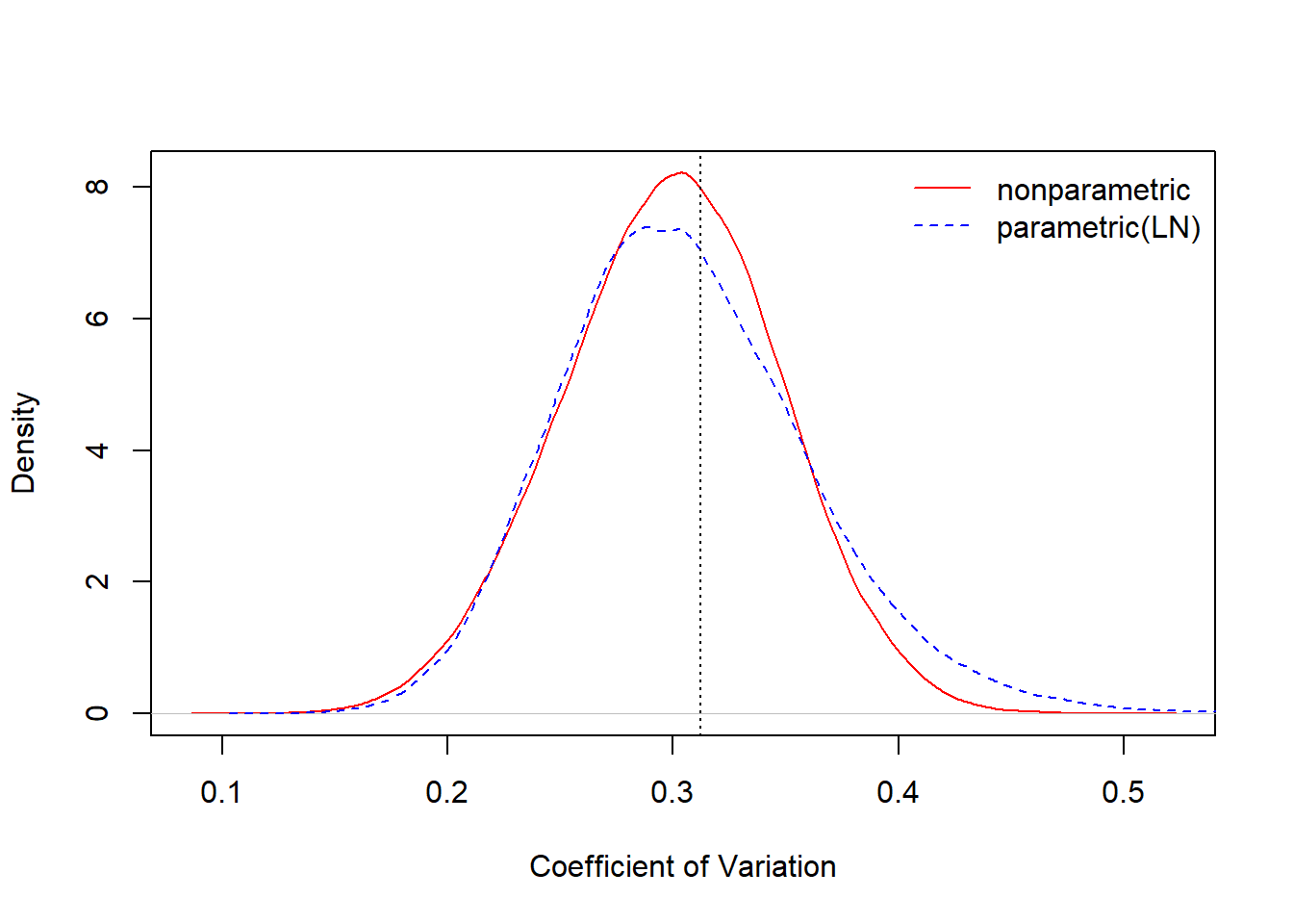
Figure 6.11: Comparision of Nonparametric and Parametric Bootstrap Distributions for the Coefficient of Variation
Example 6.2.5. Bootstrapping Censored Observations. The parametric bootstrap draws simulated realizations from a parametric estimate of the distribution function. In the same way, we can draw simulated realizations from estimates of a distribution function. As one example, we might draw from smoothed estimates of a distribution function introduced in Section 4.1.1.4. Another special case, considered here, is to draw an estimate from the Kaplan-Meier estimator introduced in Section 4.3.2.2. In this way, we can handle observations that are censored.
Specifically, return to the bodily injury data in Examples 6.2.1 and 6.2.3 but now we include the 17 claims that were censored by policy limits. In Example 4.3.6, we used this full dataset to estimate the Kaplan-Meier estimator of the survival function introduced in Section 4.3.2.2. Table 6.6 presents bootstrap estimates of the quantiles from the Kaplan-Meier survival function estimator. These include the bootstrap precision estimates, bias and standard deviation, as well as the basic 95% confidence interval.
Show R Code For Bootstrap Kaplan-Meier Estimates
Table 6.6. Bootstrap Kaplan-Meier Estimates of Quantiles at Selected Fractions
| Fraction | KM NP Estimate | Bootstrap Bias | Bootstrap SD | Lower Basic 95% CI | Upper Basic 95% CI |
|---|---|---|---|---|---|
| 0.50 | 6500 | 18.77 | 177.38 | 6067 | 6869 |
| 0.80 | 9500 | 167.08 | 429.59 | 8355 | 9949 |
| 0.90 | 12756 | 37.73 | 675.21 | 10812 | 13677 |
| 0.95 | 18500 | Inf | NaN | 12500 | 22300 |
| 0.98 | 25000 | Inf | NaN | -Inf | 27308 |
Results in Table 6.6 are consistent with the results for the uncensored subsample in Table 6.4. In Table 6.6, we note the difficulty in estimating quantiles at large fractions due to the censoring. However, for moderate size fractions (0.50, 0.80, and 0.90), the Kaplan-Meier nonparametric (KM NP) estimates of the quantile are consistent with those Table 6.4. The bootstrap standard deviation is smaller at the 0.50 (corresponding to the median) but larger at the 0.80 and 0.90 levels. The censored data analysis summarized in Table 6.6 uses more data than the uncensored subsample analysis in Table 6.4 but also has difficulty extracting information for large quantiles.
6.3 Cross-Validation
In this section, you learn how to:
- Compare and contrast cross-validation to simulation techniques and bootstrap methods.
- Use cross-validation techniques for model selection
- Explain the jackknife method as a special case of cross-validation and calculate jackknife estimates of bias and standard errors
Cross-validation, briefly introduced in Section 4.2.4, is a technique based on simulated outcomes. We now compare and contrast cross-validation to other simulation techniques already introduced in this chapter."
- Simulation, or Monte-Carlo, introduced in Section 6.1, allows us to compute expected values and other summaries of statistical distributions, such as \(p\)-values, readily.
- Bootstrap, and other resampling methods introduced in Section 6.2, provides estimators of the precision, or variability, of statistics.
- Cross-validation is important when assessing how accurately a predictive model will perform in practice.
Overlap exists but nonetheless it is helpful to think about the broad goals associated with each statistical method.
To discuss cross-validation, let us recall from Section 4.2 some of the key ideas of model validation. When assessing, or validating, a model, we look to performance measured on new data, or at least not those that were used to fit the model. A classical approach, described in Section 4.2.3, is to split the sample in two: a subpart (the training dataset) is used to fit the model and the other one (the testing dataset) is used to validate. However, a limitation of this approach is that results depend on the split; even though the overall sample is fixed, the split between training and test subsamples varies randomly. A different training sample means that model estimated parameters will differ. Different model parameters and a different test sample means that validation statistics will differ. Two analysts may use the same data and same models yet reach different conclusions about the viability of a model (based on different random splits), a frustrating situation.
6.3.1 k-Fold Cross-Validation
To mitigate this difficulty, it is common to use a cross-validation approach as introduced in Section 4.2.4. The key idea is to emulate the basic test/training approach to model validation by repeating it many times through averaging over different splits of the data. A key advantage is that the validation statistic is not tied to a specific parametric (or nonparametric) model - one can use a nonparametric statistic or a statistic that has economic interpretations - and so this can be used to compare models that are not nested (unlike likelihood ratio procedures).
Example 6.3.1. Wisconsin Property Fund. For the 2010 property fund data introduced in Section 1.3, we fit gamma and Pareto distributions to the 1,377 claims data. For details of the related goodness of fit, see Appendix Section 15.4.4. We now consider the Kolmogorov-Smirnov statistic introduced in Section 4.1.2.2. When the entire dataset was fit, the Kolmogorov-Smirnov goodness of fit statistic for the gamma distribution turns out to be 0.2639 and for the Pareto distribution is 0.0478. The lower value for the Pareto distribution indicates that this distribution is a better fit than the gamma.
To see how k-fold cross-validationA type of validation method where the data is randomly split into k groups, and each of the k groups is held out as a test dataset in turn, while the other k-1 gropus are used for distribution or model fitting, with the process repeated k times in total works, we randomly split the data into \(k=8\) groups, or folds, each having about \(1377/8 \approx 172\) observations. Then, we fit gamma and Pareto models to a data set with the first seven folds (about \(172 \cdot 7 = 1204\) observations), determine estimated parameters, and then used these fitted models with the held-out data to determine the Kolmogorov-Smirnov statistic.
Show R Code for Kolmogorov-Smirnov Cross-Validation
The results appear in Figure 6.12 where horizontal axis is Fold=1. This process was repeated for the other seven folds. The results summarized in Figure 6.12 show that the Pareto consistently provides a more reliable predictive distribution than the gamma.
# Plot the statistics
matplot(1:k,t(cvalvec),type="b", col=c(1,3), lty=1:2,
        ylim=c(0,0.4), pch = 0, xlab="Fold", ylab="KS Statistic")
legend("left", c("Pareto", "Gamma"), col=c(1,3),lty=1:2, bty="n")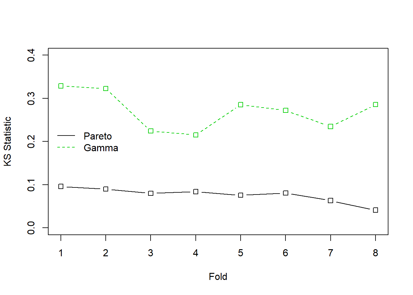
Figure 6.12: Cross Validated Kolmogorov-Smirnov (KS) Statistics for the Property Fund Claims Data. The solid black line is for the Pareto distribution, the green dashed line is for the gamma distribution. The KS statistic measures the largest deviation between the fitted distribution and the empirical distribution for each of 8 groups, or folds, of randomly selected data.
6.3.2 Leave-One-Out Cross-Validation
A special case where \(k=n\) is known as leave-one-out cross validationA special case of k-fold cross validation, where each single data point gets a turn in being the lone hold-out test data point, and n separate models in total are built and tested. This case is historically prominent and is closely related to jackknife statisticsTo calculate an estimator, leave out each observation in turn, calculate the sample estimator statistic each time, and average over the n separate estimates, a precursor of the bootstrap technique.
Even though we present it as a special case of cross-validation, it is helpful to given an explicit definition. Consider a generic statistic \(\widehat{\theta}=t(\boldsymbol{x})\) that is an estimator for a parameter of interest \(\theta\). The idea of the jackknife is to compute \(n\) values \(\widehat{\theta}_{-i}=t(\boldsymbol{x}_{-i})\), where \(\boldsymbol{x}_{-i}\) is the subsample of \(\boldsymbol{x}\) with the \(i\)-th value removed. The average of these values is denoted as \[ \overline{\widehat{\theta}}_{(\cdot)}=\frac{1}{n}\sum_{i=1}^n \widehat{\theta}_{-i} . \] These values can be used to create estimates of the bias of the statistic \(\widehat{\theta}\)
\[\begin{equation} Bias_{jack} = (n-1) \left(\overline{\widehat{\theta}}_{(\cdot)} - \widehat{\theta}\right) \tag{6.3} \end{equation}\]
as well as a standard deviation estimate
\[\begin{equation} s_{jack} =\sqrt{\frac{n-1}{n}\sum_{i=1}^n \left(\widehat{\theta}_{-i} -\overline{\widehat{\theta}}_{(\cdot)}\right)^2} ~. \tag{6.4} \end{equation}\]
Example 6.3.2. Coefficient of Variation. To illustrate, consider a small fictitious sample \(\boldsymbol{x}=\{x_1,\ldots,x_n\}\) with realizations
sample_x <- c(2.46,2.80,3.28,3.86,2.85,3.67,3.37,3.40,
              5.22,2.55,2.79,4.50,3.37,2.88,1.44,2.56,2.00,2.07,2.19,1.77)
Suppose that we are interested in the coefficient of variationStandard deviation divided by the mean of a distribution, to measure variability in terms of units of the mean \(\theta = CV = \sqrt{\mathrm{Var~}[X]}/\mathrm{E~}[X]\).
With this dataset, the estimator of the coefficient of variation turns out to be 0.31196. But how reliable is it? To answer this question, we can compute the jackknife estimates of bias and its standard deviation. The following code shows that the jackknife estimator of the bias is \(Bias_{jack} =\) -0.00627 and the jackknife standard deviation is \(s_{jack} =\) 0.01293.
CVar <- function(x) sqrt(var(x))/mean(x)
JackCVar <- function(i) sqrt(var(sample_x[-i]))/mean(sample_x[-i])
JackTheta <- Vectorize(JackCVar)(1:length(sample_x))
BiasJack <- (length(sample_x)-1)*(mean(JackTheta) - CVar(sample_x))
sd(JackTheta)
Example 6.3.3. Bodily Injury Claims and Loss Elimination Ratios. In Example 6.2.1, we showed how to compute bootstrap estimates of the bias and standard deviation for the loss elimination ratio using the Example 4.1.11 bodily injury claims data. We follow up now by providing comparable quantities using jackknife statistics.
Table 6.7 summarizes the results of the jackknife estimation. It shows that jackknife estimates of the bias and standard deviation of the loss elimination ratio \(\mathrm{E}~[\min(X,d)]/\mathrm{E}~[X]\) are largely consistent with the bootstrap methodology. Moreover, one can use the standard deviations to construct normal based confidence intervals, centered around a bias-corrected estimator. For example, at \(d=14000\), we saw in Example 4.1.11 that the nonparametric estimate of LER is 0.97678. This has an estimated bias of 0.00010, resulting in the (jackknife) bias-corrected estimator 0.97688. The 95% confidence intervals are produced by creating an interval of twice the length of 1.96 jackknife standard deviations, centered about the bias-corrected estimator (1.96 is the approximate 97.5th quantile of the standard normal distribution).
Show the R Code
Table 6.7. Jackknife Estimates of LER at Selected Deductibles
| d | NP Estimate | Bootstrap Bias | Bootstrap SD | Jackknife Bias | Jackknife SD | Lower Jackknife 95% CI | Upper Jackknife 95% CI |
|---|---|---|---|---|---|---|---|
| 4000 | 0.54113 | 0.00011 | 0.01237 | 0.00031 | 0.00061 | 0.53993 | 0.54233 |
| 5000 | 0.64960 | 0.00027 | 0.01412 | 0.00033 | 0.00068 | 0.64825 | 0.65094 |
| 10500 | 0.93563 | 0.00004 | 0.01017 | 0.00019 | 0.00053 | 0.93460 | 0.93667 |
| 11500 | 0.95281 | -0.00003 | 0.00941 | 0.00016 | 0.00047 | 0.95189 | 0.95373 |
| 14000 | 0.97678 | 0.00016 | 0.00687 | 0.00010 | 0.00034 | 0.97612 | 0.97745 |
| 18500 | 0.99382 | 0.00014 | 0.00331 | 0.00003 | 0.00017 | 0.99350 | 0.99415 |
Discussion. One of the many interesting things about the leave-one-out special case is the ability to replicate estimates exactly. That is, when the size of the fold is only one, then there is no additional uncertainty induced by the cross-validation. This means that analysts can exactly replicate work of one another, an important consideration.
Jackknife statistics were developed to understand precision of estimators, producing estimators of bias and standard deviation in equations (6.3) and (6.4). This crosses into goals that we have associated with bootstrap techniques, not cross-validation methods. This demonstrates how statistical techniques can be used to achieve different goals.
6.3.3 Cross-Validation and Bootstrap
The bootstrap is useful in providing estimators of the precision, or variability, of statistics. It can also be useful for model validation. The bootstrap approach to model validation is similar to the leave-one-out and k-fold validation procedures:
- Create a bootstrap sample by re-sampling (with replacement) \(n\) indices in \(\{1,\cdots,n\}\). That will be our training sample. Estimate the model under consideration based on this sample.
- The test, or validation sample, consists of those observations not selected for training. Evaluate the fitted model (based on the training data) using the test data.
Repeat this process many (say \(B\)) times. Take an average over the results and choose the model based on the average evaluation statistic.
Example 6.3.4. Wisconsin Property Fund. Return to Example 6.3.1 where we investigate the fit of the gamma and Pareto distributions on the property fund data. We again compare the predictive performance using the Kolmogorov-Smirnov (KS) statistic but this time using the bootstrap procedure to split the data between training and testing samples. The following provides illustrative code.
Show R Code for Bootstrapping Validation Procedures
We did the sampling using \(B=\) 100 replications. The average KS statistic for the Pareto distribution was 0.058 compared to the average for the gamma distribution, 0.262. This is consistent with earlier results and provides another piece of evidence that the Pareto is a better model for these data than the gamma.
6.4 Importance Sampling
Section 6.1 introduced Monte Carlo techniques using the inversion technique : to generate a random variable \(X\) with distribution \(F\), apply \(F^{-1}\) to calls of a random generator (uniform on the unit interval). What if we what to draw according to \(X\), conditional on \(X\in[a,b]\) ?
One can use an accept-reject mechanismA sampling method that is used where the random sample is discarded if not within a certain pre-specified range [a, b] and is commonly used when the traditional inverse transform method cannot be easily used : draw \(x\) from distribution \(F\)
- if \(x\in[a,b]\) : keep it (“accept”)
- if \(x\notin[a,b]\) : draw another one (“reject”)
Observe that from \(n\) values initially generated, we keep here only \([F(b)-F(a)]\cdot n\) draws, on average.
Example 6.4.1. Draws from a Normal Distribution. Suppose that we draw from a normal distribution with mean 2.5 and variance 1, \(N(2.5,1)\), but are only interested in draws greater that \(a \ge 2\) and less than \(b \le 4\). That is, we can only use \(F(4)-F(2) = \Phi(4-2.5)-\Phi(2-2.5)\) = 0.9332 - 0.3085 = 0.6247 proportion of the draws. Figure 6.13 demonstrates that some draws lie with the interval \((2,4)\) and some are outside.
Show R Code for Accept-Reject Mechanism
Figure 6.13: Animated Demonstration of Draws In and Outside of (2,4)
Instead, one can draw according to the conditional distribution \(F^{\star}\) defined as
\[ F^{\star}(x) = \Pr(X \le x | a < X \le b) =\frac{F(x)-F(a)}{F(b)-F(a)}, \ \ \ \text{for } a < x \le b . \]
Using the inverse transform method in Section 6.1.2, we have that the draw
\[ X^\star=F^{\star-1}\left( U \right) = F^{-1}\left(F(a)+U\cdot[F(b)-F(a)]\right) \]
has distribution \(F^{\star}\). Expressed another way, define \[ \tilde{U} = (1-U)\cdot F(a)+U\cdot F(b) \] and then use \(F^{-1}(\tilde{U})\). With this approach, each draw counts.
This can be related to the importance sampling mechanismType of sampling method where values in the region of interest can be over-sampled or values outside the region of interest can be under-sampled : we draw more frequently in regions where we expect to have quantities that have some interest. This transform can be considered as a “a change of measure.”
Show R Code for Importance Sampling by the Inverse Transform Method
In Example 6.4.1., the inverse of the normal distribution is readily available (in R, the function is qnorm). However, for other applications, this is not the case. Then, one simply uses numerical methods to determine \(X^\star\) as the solution of the equation \(F(X^\star) =\tilde{U}\) where \(\tilde{U}=(1-U)\cdot F(a)+U\cdot F(b)\). See the following illustrative code.
Show R Code for Importance Sampling via Numerical Solutions
6.5 Monte Carlo Markov Chain (MCMC)
This section is being written and is not yet complete nor edited. It is here to give you a flavor of what will be in the final version.
The idea of Monte Carlo techniques rely on the law of large numbers (that insures the convergence of the average towards the integral) and the central limit theorem (that is used to quantify uncertainty in the computations). Recall that if \((X_i)\) is an iid sequence of random variables with distribution \(F\), then
\[ \frac{1}{\sqrt{n}}\left(\sum_{i=1}^n h(X_i)-\int h(x)dF(x)\right)\overset{\mathcal{L}}{\rightarrow }\mathcal{N}(0,\sigma^2),\text{ as }n\rightarrow\infty , \] for some variance \(\sigma^2>0\). But actually, the ergodic theoremErgodic theory studies the behavior of a dynamical system when it is allowed to run for an extended time can be used to weaker the previous result, since it is not necessary to have independence of the variables. More precisely, if \((X_i)\) is a Markov ProcessA stochastic (time dependent) process that satisfies memorylessness, meaning future predictions of the process can be made solely based on its present state and not the historical path with invariant measureAny mathematical measure that is preserved by a function (the mean is an example) \(\mu\), under some additional technical assumptions, we can obtain that
\[ \frac{1}{\sqrt{n}}\left(\sum_{i=1}^n h(X_i)-\int h(x)d\mu(x)\right)\overset{\mathcal{L}}{\rightarrow }\mathcal{N}(0,\sigma_\star^2),\text{ as }n\rightarrow\infty. \] for some variance \(\sigma_\star^2>0\).
Hence, from this property, we can see that it is possible not necessarily to generate independent values from \(F\), but to generate a Markov process with invariant measure \(F\), and to consider means over the process (not necessarily independent).
Consider the case of a constrained Gaussian vector : we want to generate random pairs from a random vector \(\boldsymbol{X}\), but we are interested only in the case where the sum of the composantsComponent (smaller, self-contained part of larger entity) is large enough, which can be written \(\boldsymbol{X}^T\boldsymbol{1}> m\) for some real valued \(m\). Of course, it is possible to use the accept-reject algorithm, but we have seen that it might be quite inefficient. One can use Metropolis Hastings and Gibbs samplerA markov chain monte carlo (mcmc) method to obtain a sequence of random samples from a specified multivariate continuous probability distribution to generate a Markov process with such an invariant measure.
6.5.1 Metropolis Hastings
The algorithm is rather simple to generate from \(f\): we start with a feasible value \(x_1\). Then, at step \(t\), we need to specify a transition kernel : given \(x_t\), we need a conditional distribution for \(X_{t+1}\) given \(x_t\). The algorithm will work well if that conditional distribution can easily be simulated. Let \(\pi(\cdot|x_t)\) denote that probability.
Draw a potential value \(x_{t+1}^\star\), and \(u\), from a uniform distribution. Compute \[ R= \frac{f(x_{t+1}^\star)}{f(x_t)} \] and
- if \(u < r\), then set \(x_{t+1}=x_t^\star\)
- if \(u\leq r\), then set \(x_{t+1}=x_t\)
Here \(r\) is called the acceptance-ratio: we accept the new value with probability \(r\) (or actually the smallest between \(1\) and \(r\) since \(r\) can exceed \(1\)).
For instance, assume that \(f(\cdot|x_t)\) is uniform on \([x_t-\varepsilon,x_t+\varepsilon]\) for some \(\varepsilon>0\), and where \(f\) (our target distribution) is the \(\mathcal{N}(0,1)\). We will never draw from \(f\), but we will use it to compute our acceptance ratio at each step.
Show R Code
In the code above, vec contains values of \(\boldsymbol{x}=(x_1,x_2,\cdots)\), innov is the innovation.
Show R Code
Now, if we use more simulations, we get
vec <- metrop1(10000)
simx <- vec[1000:10000,1]
par(mfrow=c(1,4))
plot(simx,type="l")
hist(simx,probability = TRUE,col="light blue",border="white")
lines(u,dnorm(u),col="red")
qqnorm(simx)
acf(simx,lag=100,lwd=2,col="light blue")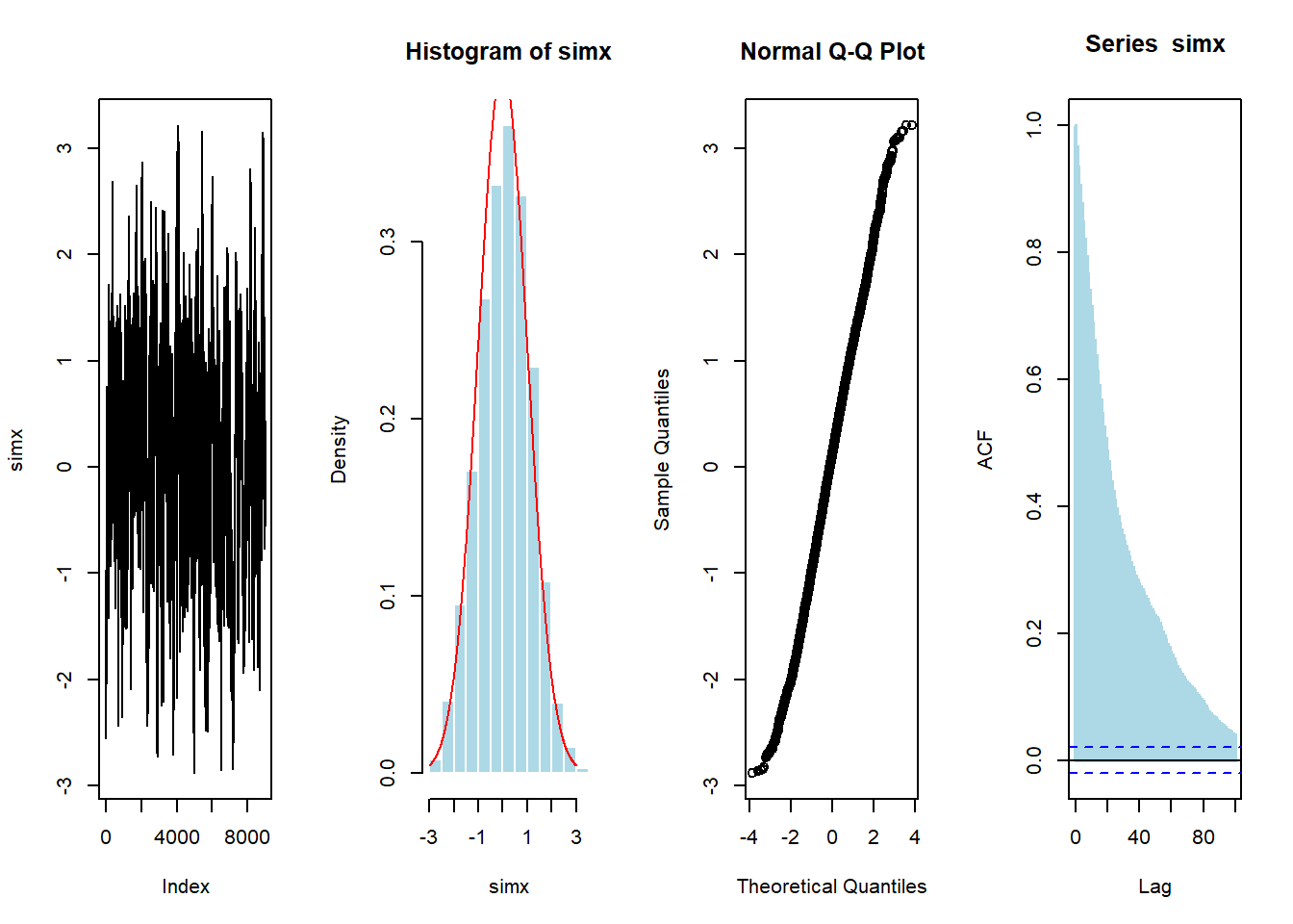
6.5.2 Gibbs Sampler
Consider some vector \(\boldsymbol{X}=(X_1,\cdots,X_d)\) with independent components, \(X_i \sim \mathcal{E}(\lambda_i)\). We sample to sample from \(\boldsymbol{X}\) given \(\boldsymbol{X}^T\boldsymbol{1}>s\) for some threshold \(s>0\).
- with some starting point \(\boldsymbol{x}_0\),
- pick up (randomly) \(i\in\{1,\cdots,d\}\)
- \(X_i\) given \(X_i > s-\boldsymbol{x}_{(-i)}^T\boldsymbol{1}\) has an Exponential distribution \(\mathcal{E}(\lambda_i)\)
- draw \(Y\sim \mathcal{E}(\lambda_i)\) and set \(x_i=y +(s-\boldsymbol{x}_{(-i)}^T\boldsymbol{1})_+\) until \(\boldsymbol{x}_{(-i)}^T\boldsymbol{1}+x_i>s\)
Show R Code
plot(sim,xlim=c(1,11),ylim=c(0,4.3))
polygon(c(-1,-1,6),c(-1,6,-1),col="red",density=15,border=NA)
abline(5,-1,col="red")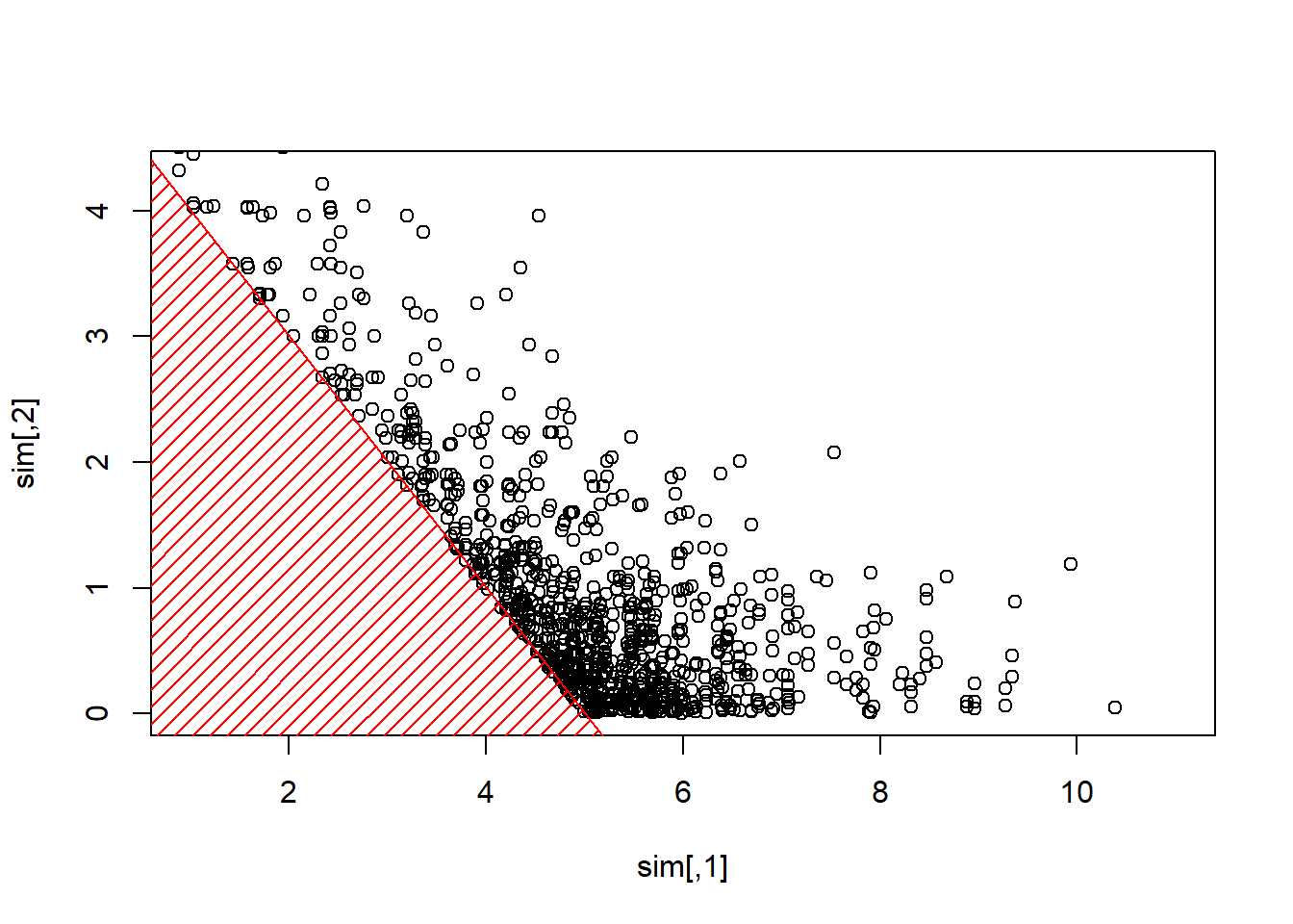
The construction of the sequence (MCMCMarkov Chain Monte Carlo algorithms are iterative) can be visualized below
Show R Code
6.6 Further Resources and Contributors
- Include historical references for jackknife (Quenouille, Tukey, Efron)
- Here are some links to learn more about reproducibility and randomness and how to go from a random generator to a sample function.
Contributors
- Arthur Charpentier, Université du Quebec á Montreal, and Edward W. (Jed) Frees, University of Wisconsin-Madison, are the principal authors of the initial version of this chapter. Email: jfrees@bus.wisc.edu and/or arthur.charpentier@gmail.com for chapter comments and suggested improvements.
- Chapter reviewers include Yvonne Chueh and Brian Hartman. Write Jed or Arthur to add you name here.
6.6.1 TS 6.A. Bootstrap Applications in Predictive Modeling
This section is under construction.