Chapter 3 Modeling Loss Severity

Chapter Preview. The traditional loss distribution approach to modeling aggregate lossesAggregate claims, or total claims observed in the time period starts by separately fitting a frequency distribution to the number of losses and a severity distribution to the size of losses. The estimated aggregate loss distribution combines the loss frequency distribution and the loss severity distribution by convolution. Discrete distributions often referred to as counting or frequency distributions were used in Chapter 2 to describe the number of events such as number of accidents to the driver or number of claims to the insurer. Lifetimes, asset values, losses and claim sizes are usually modeled as continuous random variables and as such are modeled using continuous distributions, often referred to as loss or severity distributions. A mixture distributionA weighted average of other distributions, which may be continuous or discrete is a weighted combination of simpler distributions that is used to model phenomenon investigated in a heterogeneous population, such as modeling more than one type of claims in liability insuranceInsurance that compensates an insured for loss due to legal liability towards others (small frequent claims and large relatively rare claims). In this chapter we explore the use of continuous as well as mixture distributions to model the random size of loss. Sections 3.1 and 3.2 present key attributes that characterize continuous models and means of creating new distributions from existing ones. Section 3.4 describes the effect of coverage modifications, which change the conditions that trigger a payment, such as applying deductibles, limits, or adjusting for inflation, on the distribution of individual loss amounts. For calibrating models, Section 3.5 deepens our understanding of maximum likelihood methods. The frequency distributions from Chapter 2 will be combined with the ideas from this chapter to describe the aggregate losses over the whole portfolio in Chapter 5.

3.1 Basic Distributional Quantities

---

In this section, you learn how to define some basic distributional quantities:

• moments,
• percentiles, and
• generating functions.

---

3.1.1 Moments

Let \(X\) be a continuous random variableRandom variable which can take infinitely many values in its specified domain with probability density function (pdf) \(f_{X}\left( x \right)\) and distribution function \(F_{X}\left( x \right)\). The k-th raw momentThe kth moment of a random variable x is the average (expected) value of x^k of \(X\), denoted by \(\mu_{k}^{\prime}\), is the expected valueAverage of the k-th power of \(X\), provided it exists. The first raw moment \(\mu_{1}^{\prime}\) is the mean of \(X\) usually denoted by \(\mu\). The formula for \(\mu_{k}^{\prime}\) is given as \[ \mu_{k}^{\prime} = \mathrm{E}\left( X^{k} \right) = \int_{0}^{\infty}{x^{k}f_{X}\left( x \right)dx } . \] The support of the random variable \(X\) is assumed to be nonnegative since actuarial phenomena are rarely negative. For example, an easy integration by parts shows that the raw moments for nonnegative variables can also be computed using \[ \mu_{k}^{\prime} = \int_{0}^{\infty}{k~x^{k-1}\left[1- F_{X}(x) \right]dx }, \] that is based on the survival function, denoted as \(S_X(x) = 1-F_{X}(x)\). This formula is particularly useful when \(k=1\). Section 3.4.2 discusses this approach in more detail.

The k-th central momentThe kth central moment of a random variable x is the expected value of (x-its mean)^k of \(X\), denoted by \(\mu_{k}\), is the expected value of the k-th power of the deviation of \(X\) from its mean \(\mu\). The formula for \(\mu_{k}\) is given as \[ \mu_{k} = \mathrm{E}\left\lbrack {(X - \mu)}^{k} \right\rbrack = \int_{0}^{\infty}{\left( x - \mu \right)^{k}f_{X}\left( x \right) dx }. \] The second central moment \(\mu_{2}\) defines the varianceSecond central moment of a random variable x, measuring the expected squared deviation of between the variable and its mean of \(X\), denoted by \(\sigma^{2}\). The square root of the variance is the standard deviationThe square-root of variance \(\sigma\).

From a classical perspective, further characterization of the shape of the distribution includes its degree of symmetry as well as its flatness compared to the normal distribution. The ratio of the third central moment to the cube of the standard deviation \(\left( \mu_{3} / \sigma^{3} \right)\) defines the coefficient of skewnessMeasure of the symmetry of a distribution, 3rd central moment/standard deviation^3 which is a measure of symmetry. A positive coefficient of skewness indicates that the distribution is skewed to the right (positively skewed). The ratio of the fourth central moment to the fourth power of the standard deviation \(\left(\mu_{4} / \sigma^{4} \right)\) defines the coefficient of kurtosisMeasure of the peaked-ness of a distribution, 4th central moment/standard deviation^4. The normal distribution has a coefficient of kurtosis of 3. Distributions with a coefficient of kurtosis greater than 3 have heavier tails than the normal, whereas distributions with a coefficient of kurtosis less than 3 have lighter tails and are flatter. Section 10.2 describes the tails of distributions from an insurance and actuarial perspective.

Example 3.1.1. Actuarial Exam Question. Assume that the rvRandom variable \(X\) has a gamma distribution with mean 8 and skewness 1. Find the variance of \(X\). (Hint: The gamma distribution is reviewed in Section 3.2.1.)

Show Example Solution

Solution. The pdf of \(X\) is given by

\[ f_{X}\left( x \right) = \frac{\left( x / \theta \right)^{\alpha}}{x ~\Gamma\left( \alpha \right)} e^{- x / \theta} \] for \(x > 0\). For \(\alpha>0\), the k-th raw moment is

\[ \mu_{k}^{\prime} = \mathrm{E}\left( X^{k} \right) = \int_{0}^{\infty}{\frac{1}{\Gamma\left( \alpha \right)\theta^{\alpha}}x^{k + \alpha - 1}e^{- x / \theta} dx} = \frac{\Gamma\left( k + \alpha \right)}{\Gamma\left( \alpha \right)}\theta^{k} \] Given \(\Gamma\left( r + 1 \right) = r\Gamma\left( r \right)\) and \(\Gamma\left( 1 \right) = 1\), then \(\mu_{1}^{\prime} = \mathrm{E}\left( X \right) = \alpha\theta\), \(\mu_{2}^{\prime} = \mathrm{E}\left( X^{2} \right) = \left( \alpha + 1 \right)\alpha\theta^{2}\), \(\mu_{3}^{\prime} = \mathrm{E}\left( X^{3} \right) = \left( \alpha + 2 \right)\left( \alpha + 1 \right)\alpha\theta^{3}\), and \(\mathrm{Var}\left( X \right) = (\alpha + 1)\alpha\theta^2 - (\alpha\theta)^2 = \alpha\theta^{2}\).

\[ \begin{array}{ll} \text{Skewness} &= \frac{\mathrm{E}\left\lbrack {(X - \mu_{1}^{\prime})}^{3} \right\rbrack}{{\left( \mathrm{Var}X \right)}^{3/2}} = \frac{\mu_{3}^{\prime} - 3\mu_{2}^{\prime}\mu_{1}^{\prime} + 2{\mu_{1}^{\prime}}^{3}}{{\left(\mathrm{Var} X \right)}^{3/2}} \\ &= \frac{\left( \alpha + 2 \right)\left( \alpha + 1 \right)\alpha\theta^{3} - 3\left( \alpha + 1 \right)\alpha^{2}\theta^{3} + 2\alpha^{3}\theta^{3}}{\left( \alpha\theta^{2} \right)^{3/2}} \\ &= \frac{2}{\alpha^{1/2}} = 1. \end{array} \]

Hence, \(\alpha = 4\). Since, \(\mathrm{E}\left( X \right) = \alpha\theta = 8\), then \(\theta = 2\) and finally, \(\mathrm{Var}\left( X \right) = \alpha\theta^{2} = 16\).

---

3.1.2 Quantiles

Quantiles can also be used to describe the characteristics of the distribution of \(X\). When the distribution of \(X\) is continuous, for a given fraction \(0 \leq p \leq 1\) the corresponding quantile is the solution of the equation \[ F_{X}\left( \pi_{p} \right) = p . \] For example, the middle point of the distribution, \(\pi_{0.5}\), is the median50th percentile of a definition, or middle value where half of the distribution lies below. A percentileThe pth percentile of a random variable x is the smallest value x_p such that the probability of not exceeding it is p% is a type of quantile; a \(100p\) percentile is the number such that \(100 \times p\) percent of the data is below it.

Example 3.1.1. Actuarial Exam Question. Let \(X\) be a continuous random variable with density function \(f_{X}\left( x \right) = \theta e^{- \theta x}\), for \(x > 0\) and 0 elsewhere. If the median of this distribution is \(\frac{1}{3}\), find \(\theta\).

Show Example Solution

Solution.

The distribution function is \(F_{X}\left( x \right) = 1 - e^{- \theta x}\). So, \(F_{X}\left( \pi_{0.5} \right) = 1 - e^{- \theta\pi_{0.5}} = 0.5\). As, \(\pi_{0.5} = \frac{1}{3}\), we have \(F_X\left(\frac{1}{3}\right) = 1 - e^{-\theta / 3} = 0.5\) and \(\theta = 3 \log 2\).

---

Section 4.1.1.3 will extend the definition of quantiles to include distributions that are discrete, continuous, or a hybrid combination.

3.1.3 Moment Generating Function

The moment generating function (mgf)The mgf of random variable n is defined the expectation of exp(tn), as a function of t, denoted by \(M_{X}(t)\) uniquely characterizes the distribution of \(X\). While it is possible for two different distributions to have the same moments and yet still differ, this is not the case with the moment generating function. That is, if two random variables have the same moment generating function, then they have the same distribution. The moment generating function is given by \[ M_{X}(t) = \mathrm{E}\left( e^{tX} \right) = \int_{0}^{\infty}{e^{\text{tx}}f_{X}\left( x \right) dx } \] for all \(t\) for which the expected value exists. The mgf is a real function whose k-th derivative at zero is equal to the k-th raw moment of \(X\). In symbols, this is \[ \left.\frac{d^k}{dt^k} M_{X}(t)\right|_{t=0} = \mathrm{E}\left( X^{k} \right) . \]

Example 3.1.3. Actuarial Exam Question. The random variable \(X\) has an exponential distribution with mean \(\frac{1}{b}\). It is found that \(M_{X}\left( - b^{2} \right) = 0.2\). Find \(b\). (Hint: The exponential is a special case of the gamma distribution which is reviewed in Section 3.2.1.)

Show Example Solution

Solution.

With \(X\) having an exponential distribution with mean \(\frac{1}{b}\), we have that \[ M_{X}(t) = \mathrm{E}\left( e^{tX} \right) = \int_{0}^{\infty}{e^{\text{tx}}be^{- bx} dx} = \int_{0}^{\infty}{be^{- x\left( b - t \right)} dx} = \frac{b}{\left( b - t \right)}. \]

Then, \[ M_{X}\left( - b^{2} \right) = \frac{b}{\left( b + b^{2} \right)} = \frac{1}{\left( 1 + b \right)} = 0.2. \] Thus, \(b = 4\).

---

Example 3.1.4. Actuarial Exam Question. Let \(X_{1}, \ldots, X_{n}\) be independentTwo variables are independent if conditional information given about one variable provides no information regarding the other variable random variables, where \(X_i\) has a gamma distribution with parameters \(\alpha_{i}\) and \(\theta\). Find the distribution of \(S = \sum_{i = 1}^{n}X_{i}\), the mean \(\mathrm{E}(S)\), and the variance \(\mathrm{Var}(S)\).

Show Example Solution

Solution.

The mgf of \(S\) is \[ M_{S}(t) = \text{E}\left( e^{\text{tS}} \right) = \mathrm{E}\left( e^{t\sum_{i = 1}^{n}X_{i}} \right) = \mathrm{E}\left( \prod_{i = 1}^{n}e^{tX_{i}} \right) . \] Using independence, we get
\[ M_{S}(t) = \prod_{i = 1}^{n}{\mathrm{E}\left( e^{tX_{i}} \right) = \prod_{i = 1}^{n}{M_{X_{i}}(t)}} . \]

The moment generating function of the gamma distribution \(X_i\) is \(M_{X_i}(t) = (1-\theta t)^{\alpha_i}\). Then, \[ M_{S}(t) = \prod_{i = 1}^{n}\left( 1 - \theta t \right)^{- \alpha_{i}} = \left( 1 - \theta t \right)^{- \sum_{i = 1}^{n}\alpha_{i}} . \] This indicates that the distribution of \(S\) is gamma with parameters \(\sum_{i = 1}^{n}\alpha_{i}\) and \(\theta\).

This is a demonstration of how we can use the uniqueness property of the moment generating function to determine the probability distribution of a function of random variables.

We can find the mean and variance from the properties of the gamma distribution. Alternatively, by finding the first and second derivatives of \(M_{S}(t)\) at zero, we can show that \(\mathrm{E}\left( S \right) = \left. \ \frac{\partial M_{S}(t)}{\partial t} \right|_{t = 0} = \alpha\theta\) where \(\alpha = \sum_{i = 1}^{n}\alpha_{i}\), and

\[ \mathrm{E}\left( S^{2} \right) = \left. \ \frac{\partial^{2}M_{S}(t)}{\partial t^{2}} \right|_{t = 0} = \left( \alpha + 1 \right)\alpha\theta^{2}. \] Hence, \(\mathrm{Var}\left( S \right) = \alpha\theta^{2}\).

---

One can also use the moment generating function to compute the probability generating function

\[ P_{X}(z) = \mathrm{E}\left( z^{X} \right) = M_{X}\left( \log z \right) . \]

As introduced in Section 2.2.2, the probability generating function is more useful for discrete random variables.

Show Quiz Solution

---

3.2 Continuous Distributions for Modeling Loss Severity

---

In this section, you learn how to define and apply four fundamental severity distributions:

• gamma,
• Pareto,
• Weibull, and
• generalized beta distribution of the second kind.

---

3.2.1 Gamma Distribution

Recall that the traditional approach in modeling losses is to fit separate models for frequency and claim severity. When frequency and severity are modeled separately it is common for actuaries to use the Poisson distribution (introduced in Section 2.2.3.2) for claim count and the gamma distribution to model severity. An alternative approach for modeling losses that has recently gained popularity is to create a single model for pure premium (average claim cost) that will be described in Chapter 4.

The continuous variable \(X\) is said to have the gamma distribution with shape parameter \(\alpha\) and scale parameter \(\theta\) if its probability density function is given by \[ f_{X}\left( x \right) = \frac{\left( x/ \theta \right)^{\alpha}}{x~ \Gamma\left( \alpha \right)}\exp \left( -x/ \theta \right) \ \ \ \text{for } x > 0 . \] Note that \(\alpha > 0,\ \theta > 0\).

The two panels in Figure 3.1 demonstrate the effect of the scale and shape parameters on the gamma density function.

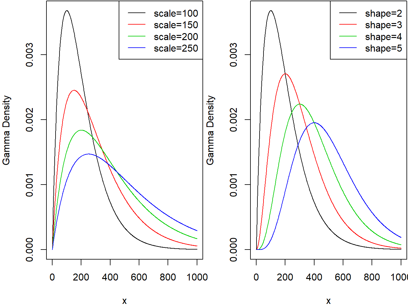
Figure 3.1: Gamma Densities. The left-hand panel is with shape=2 and varying scale. The right-hand panel is with scale=100 and varying shape.

R Code for Gamma Density Plots

par(mfrow=c(1, 2), mar = c(4, 4, .1, .1))

# Varying Scale Gamma Densities
scaleparam <- seq(100, 250, by = 50)
shapeparam <- 2:5
x <- seq(0, 1000, by = 1)
fgamma <- dgamma(x, shape = 2, scale = scaleparam[1])
plot(x, fgamma, type = "l", ylab = "Gamma Density")
for(k in 2:length(scaleparam)){
  fgamma <- dgamma(x,shape = 2, scale = scaleparam[k])
  lines(x,fgamma, col = k)
}
legend("topright", c("scale=100", "scale=150", "scale=200", "scale=250"), lty=1, col = 1:4)

# Varying Shape Gamma Densities
fgamma <- dgamma(x, shape = shapeparam[1], scale = 100)
plot(x, fgamma, type = "l", ylab = "Gamma Density")
for(k in 2:length(shapeparam)){
  fgamma <- dgamma(x,shape = shapeparam[k], scale = 100)
  lines(x,fgamma, col = k)
}
legend("topright", c("shape=2", "shape=3", "shape=4", "shape=5"), lty=1, col = 1:4)

When \(\alpha = 1\) the gamma reduces to an exponential distributionA single parameter continous probability distribution that is defined by its rate parameter and when \(\alpha = \frac{n}{2}\) and \(\theta = 2\) the gamma reduces to a chi-square distributionA common distribution used in chi-square tests for determining goodness of fit of observed data to a theorized distribution with \(n\) degrees of freedom. As we will see in Section 15.4, the chi-square distribution is used extensively in statistical hypothesis testing.

The distribution function of the gamma model is the incomplete gamma function, denoted by \(\Gamma\left(\alpha; \frac{x}{\theta} \right)\), and defined as \[ F_{X}\left( x \right) = \Gamma\left( \alpha; \frac{x}{\theta} \right) = \frac{1}{\Gamma\left( \alpha \right)}\int_{0}^{x /\theta}t^{\alpha - 1}e^{- t}~dt , \] with \(\alpha > 0,\ \theta > 0\). For an integer \(\alpha\), it can be written as \(\Gamma\left( \alpha; \frac{x}{\theta} \right) = 1 - e^{-x/\theta}\sum_{k = 0}^{\alpha-1}\frac{(x/\theta)^k}{k!}\).

The \(k\)-th raw moment of the gamma distributed random variable for any positive \(k\) is given by \[ \mathrm{E}\left( X^{k} \right) = \theta^{k} \frac{\Gamma\left( \alpha + k \right)}{\Gamma\left( \alpha \right)} . \] The mean and variance are given by \(\mathrm{E}\left( X \right) = \alpha\theta\) and \(\mathrm{Var}\left( X \right) = \alpha\theta^{2}\), respectively.

Since all moments exist for any positive \(k\), the gamma distribution is considered a light tailed distributionA distribution with thinner tails than the benchmark exponential distribution, which may not be suitable for modeling risky assets as it will not provide a realistic assessment of the likelihood of severe losses.

3.2.2 Pareto Distribution

The Pareto distributionA heavy-tailed and positively skewed distribution with 2 parameters, named after the Italian economist Vilfredo Pareto (1843-1923), has many economic and financial applications. It is a positively skewed and heavy-tailed distribution which makes it suitable for modeling income, high-risk insurance claims and severity of large casualty losses. The survival function of the Pareto distribution which decays slowly to zero was first used to describe the distribution of income where a small percentage of the population holds a large proportion of the total wealth. For extreme insurance claims, the tail of the severity distribution (losses in excess of a threshold) can be modeled using a Generalized Pareto distribution.

The continuous variable \(X\) is said to have the (two parameter) Pareto distribution with shape parameter \(\alpha\) and scale parameter \(\theta\) if its pdfProbability density function is given by

\[\begin{equation} f_{X}\left( x \right) = \frac{\alpha\theta^{\alpha}}{\left( x + \theta \right)^{\alpha + 1}} \ \ \ x > 0, \ \alpha > 0, \ \theta > 0. \tag{3.1} \end{equation}\]

The two panels in Figure 3.2 demonstrate the effect of the scale and shape parameters on the Pareto density function. There are other formulations of the Pareto distribution including a one parameter version given in Appendix Section 18.2. Henceforth, when we refer the Pareto distribution, we mean the version given through the pdf in equation (3.1).

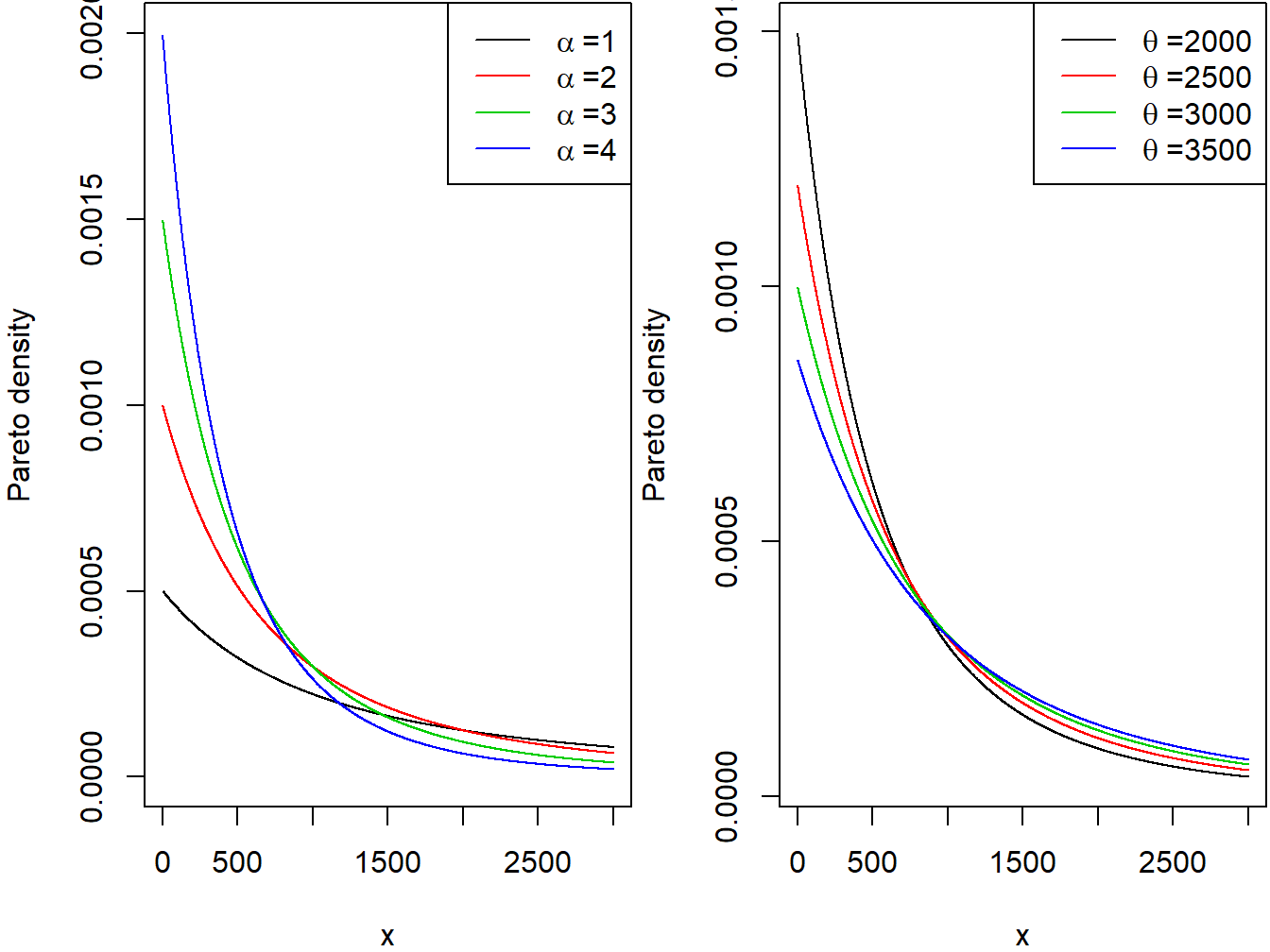
Figure 3.2: Pareto Densities. The left-hand panel is with scale=2000 and varying shape. The right-hand panel is with shape=3 and varying scale.

R Code for Pareto Density Plots

par(mfrow=c(1, 2), mar = c(4, 4, .1, .1))

# Varying Scale Pareto Densities
x <- seq(1, 3000, by = 1)
scaleparam <- seq(2000, 3500, 500)
shapeparam <- 1:4

# varying the shape parameter
plot(x, actuar::dpareto(x, shape = shapeparam[1], scale = 2000), ylim=c(0,0.002),type = "l", ylab = "Pareto density")
for(k in 2:length(shapeparam)){
  lines(x, actuar::dpareto(x, shape = shapeparam[k], scale = 2000), col = k)
}
legend("topright", c(expression(alpha~'=1'), expression(alpha~'=2'), expression(alpha~'=3'), expression(alpha~'=4')), lty=1, col = 1:4)

# Varying Shape Pareto Densities
plot(x, actuar::dpareto(x, shape = 3, scale = scaleparam[1]), type = "l", ylab = "Pareto density")
for(k in 2:length(scaleparam)){
  lines(x, actuar::dpareto(x, shape = 3, scale = scaleparam[k]), col = k)
}
legend("topright", c(expression(theta~'=2000'), expression(theta~'=2500'), expression(theta~'=3000'), expression(theta~'=3500')), lty=1, col = 1:4)

The distribution function of the Pareto distribution is given by \[ F_{X}\left( x \right) = 1 - \left( \frac{\theta}{x + \theta} \right)^{\alpha} \ \ \ x > 0,\ \alpha > 0,\ \theta > 0. \]

It can be easily seen that the hazard functionRatio of the probability density function and the survival function: f(x)/s(x), and represents an instantaneous probability within a small time frame of the Pareto distribution is a decreasing function in \(x\), another indication that the distribution is heavy tailed. Again using the analogy of the income of a population, when the hazard function decreases over time the population dies off at a decreasing rate resulting in a heavier tail for the distribution. The hazard function reveals information about the tail distribution and is often used to model data distributions in survival analysis. The hazard function is defined as the instantaneous potential that the event of interest occurs within a very narrow time frame.

The \(k\)-th raw moment of the Pareto distributed random variable exists, if and only if, \(\alpha > k\). If \(k\) is a positive integer then \[ \mathrm{E}\left( X^{k} \right) = \frac{\theta^{k}~ k!}{\left( \alpha - 1 \right)\cdots\left( \alpha - k \right)} \ \ \ \alpha > k. \] The mean and variance are given by \[\mathrm{E}\left( X \right) = \frac{\theta}{\alpha - 1} \ \ \ \text{for } \alpha > 1\] and \[\mathrm{Var}\left( X \right) = \frac{\alpha\theta^{2}}{\left( \alpha - 1 \right)^{2}\left( \alpha - 2 \right)} \ \ \ \text{for } \alpha > 2,\]respectively.

Example 3.2.1. The claim size of an insurance portfolio follows the Pareto distribution with mean and variance of 40 and 1800, respectively. Find

1. The shape and scale parameters.
2. The 95-th percentile of this distribution.

Show Example Solution

Solution.

a. As, \(X\sim Pa(\alpha,\theta)\), we have \(\mathrm{E}\left( X \right) = \frac{\theta}{\alpha - 1} = 40\) and \(\mathrm{Var}\left( X \right) = \frac{\alpha\theta^{2}}{\left( \alpha - 1 \right)^{2}\left( \alpha - 2 \right)} = 1800\). By dividing the square of the first equation by the second we get \(\frac{\alpha - 2}{\alpha} = \frac{40^{2}}{1800}\). Thus, \(\alpha = 18.02\) and \(\theta = 680.72\).
b. The 95-th percentile, \(\pi_{0.95}\), satisfies the equation \[ F_{X}\left( \pi_{0.95} \right) = 1 - \left( \frac{680.72}{\pi_{0.95} + 680.72} \right)^{18.02} = 0.95. \] Thus, \(\pi_{0.95} = 122.96\).

---

3.2.3 Weibull Distribution

The Weibull distributionA positively skewed continuous distribution with 2 parameters that can have an increasing or decreasing hazard function depending on the shape parameter, named after the Swedish physicist Waloddi Weibull (1887-1979) is widely used in reliability, life data analysis, weather forecasts and general insurance claims. Truncated data arise frequently in insurance studies. The Weibull distribution has been used to model excess of loss treaty over automobile insurance as well as earthquake inter-arrival times.

The continuous variable \(X\) is said to have the Weibull distribution with shape parameter \(\alpha\) and scale parameter \(\theta\) if its pdf is given by \[ f_{X}\left( x \right) = \frac{\alpha}{\theta}\left( \frac{x}{\theta} \right)^{\alpha - 1} \exp \left(- \left( \frac{x}{\theta} \right)^{\alpha}\right) \ \ \ x > 0,\ \alpha > 0,\ \theta > 0. \] The two panels in Figure 3.3 demonstrate the effects of the scale and shape parameters on the Weibull density function.

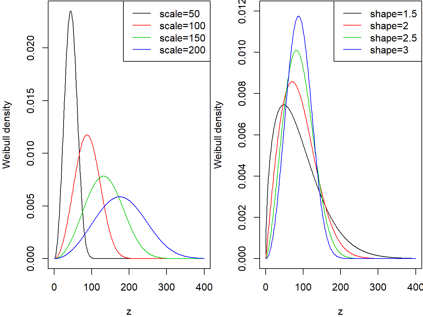
Figure 3.3: Weibull Densities. The left-hand panel is with shape=3 and varying scale. The right-hand panel is with scale=100 and varying shape.

R Code for Weibull Density Plots

par(mfrow=c(1, 2), mar = c(4, 4, .1, .1))

# Varying Scale Weibull Densities
z<- seq(0,400,by=1)
scaleparam <- seq(50,200,50)
shapeparam <- seq(1.5,3,0.5)
plot(z, dweibull(z, shape = 3, scale = scaleparam[1]), type = "l", ylab = "Weibull density")
for(k in 2:length(scaleparam)){
  lines(z,dweibull(z,shape = 3, scale = scaleparam[k]), col = k)}
legend("topright", c("scale=50", "scale=100", "scale=150", "scale=200"), lty=1, col = 1:4)

# Varying Shape Weibull Densities
plot(z, dweibull(z, shape = shapeparam[1], scale = 100), ylim=c(0,0.012), type = "l", ylab = "Weibull density")
for(k in 2:length(shapeparam)){
  lines(z,dweibull(z,shape = shapeparam[k], scale = 100), col = k)}
legend("topright", c("shape=1.5", "shape=2", "shape=2.5", "shape=3"), lty=1, col = 1:4)

The distribution function of the Weibull distribution is given by \[ F_{X}\left( x \right) = 1 - \exp\left(- \left( \frac{x}{\theta} \right)^{\alpha}~\right) \ \ \ x > 0,\ \alpha > 0,\ \theta > 0. \]

It can be easily seen that the shape parameter \(\alpha\) describes the shape of the hazard function of the Weibull distribution. The hazard function is a decreasing function when \(\alpha < 1\) (heavy tailed distribution), constant when \(\alpha = 1\) and increasing when \(\alpha > 1\) (light tailed distribution). This behavior of the hazard function makes the Weibull distribution a suitable model for a wide variety of phenomena such as weather forecasting, electrical and industrial engineering, insurance modeling, and financial risk analysis.

The \(k\)-th raw moment of the Weibull distributed random variable is given by \[ \mathrm{E}\left( X^{k} \right) = \theta^{k}~\Gamma\left( 1 + \frac{k}{\alpha} \right) . \]

The mean and variance are given by \[ \mathrm{E}\left( X \right) = \theta~\Gamma\left( 1 + \frac{1}{\alpha} \right) \] and \[ \mathrm{Var}(X)= \theta^{2}\left( \Gamma\left( 1 + \frac{2}{\alpha} \right) - \left\lbrack \Gamma\left( 1 + \frac{1}{\alpha} \right) \right\rbrack ^{2}\right), \] respectively.

Example 3.2.2. Suppose that the probability distribution of the lifetime of AIDS patients (in months) from the time of diagnosis is described by the Weibull distribution with shape parameter 1.2 and scale parameter 33.33.

1. Find the probability that a randomly selected person from this population survives at least 12 months.
2. A random sample of 10 patients will be selected from this population. What is the probability that at most two will die within one year of diagnosis.
3. Find the 99-th percentile of the distribution of lifetimes.

Show Example Solution

Solution.

a. Let \(X\) be the lifetime of AIDS patients (in months) having a Weibull distribution with parameters \(\left( 1.2,33.33 \right)\). We have,

\[ \Pr \left( X \geq 12 \right) = S_{X} \left( 12 \right) = e^{- \left( \frac{12}{33.33} \right)^{1.2}} = 0.746. \]

b. Let \(Y\) be the number of patients who die within one year of diagnosis. Then, \(Y\sim Bin\left( 10,\ 0.254 \right)\) and \(\Pr\left( Y \leq 2 \right) = 0.514.\)

c. Let \(\pi_{0.99}\) denote the 99-th percentile of this distribution. Then, \[ S_{X}\left( \pi_{0.99} \right) = \exp\left\{- \left( \frac{\pi_{0.99}}{33.33} \right)^{1.2}\right\} = 0.01. \] Solving for \(\pi_{0.99}\), we get \(\pi_{0.99} = 118.99\).

---

3.2.4 The Generalized Beta Distribution of the Second Kind

The Generalized Beta Distribution of the Second KindA 4-parameter flexible distribution that encompasses many common distributions (GB2) was introduced by Venter (1983) in the context of insurance loss modeling and by McDonald (1984) as an income and wealth distribution. It is a four-parameter, very flexible, distribution that can model positively as well as negatively skewed distributions.

The continuous variable \(X\) is said to have the GB2 distribution with parameters \(\sigma\), \(\theta\), \(\alpha_1\) and \(\alpha_2\) if its pdf is given by

\[\begin{equation} f_{X}\left( x \right) = \frac{(x/\theta)^{\alpha_2/\sigma}}{x \sigma~\mathrm{B}\left( \alpha_1,\alpha_2\right)\left\lbrack 1 + \left( x/\theta \right)^{1/\sigma} \right\rbrack^{\alpha_1 + \alpha_2}} \ \ \ \text{for } x > 0, \tag{3.2} \end{equation}\]

\(\sigma,\theta,\alpha_1,\alpha_2 > 0\), and where the beta function \(\mathrm{B}\left( \alpha_1,\alpha_2 \right)\) is defined as

\[ \mathrm{B}\left( \alpha_1,\alpha_2\right) = \int_{0}^{1}{t^{\alpha_1 - 1}\left( 1 - t \right)^{\alpha_2 - 1}}~ dt. \]

The GB2 provides a model for heavy as well as light tailed data. It includes the exponential, gamma, Weibull, Burr, Lomax, F, chi-square, Rayleigh, lognormal and log-logistic as special or limiting cases. For example, by setting the parameters \(\sigma = \alpha_1 = \alpha_2 = 1\), the GB2 reduces to the log-logistic distribution. When \(\sigma = 1\) and \(\alpha_2 \rightarrow \infty\), it reduces to the gamma distribution, and when \(\alpha = 1\) and \(\alpha_2 \rightarrow \infty\), it reduces to the Weibull distribution.

A GB2 random variable can be constructed as follows. Suppose that \(G_1\) and \(G_2\) are independent random variables where \(G_i\) has a gamma distribution with shape parameter \(\alpha_i\) and scale parameter 1. Then, one can show that the random variable \(X = \theta \left(\frac{G_1}{G_2}\right)^{\sigma}\) has a GB2 distribution with pdf summarized in equation (3.2). This theoretical result has several implications. For example, when the moments exist, one can show that the \(k\)-th raw moment of the GB2 distributed random variable is given by

\[ \mathrm{E}\left( X^{k} \right) = \frac{\theta^{k}~\mathrm{B}\left( \alpha_1 +k \sigma,\alpha_2 - k \sigma \right)}{\mathrm{B}\left( \alpha_1,\alpha_2 \right)}, \ \ \ k > 0. \]

As will be described in Section 3.3.3, the GB2 is also related to an \(F\)-distribution, a result that can be useful in simulation and residual analysis.

Earlier applications of the GB2 were on income data and more recently have been used to model long-tailed claims data (Section 10.2 describes different interpretations of the descriptor “long-tail”). The GB2 has been used to model different types of automobile insurance claims, severity of fire losses, as well as medical insurance claim data.

Show Quiz Solution

---

3.3 Methods of Creating New Distributions

---

In this section, you learn how to:

• Understand connections among the distributions
• Give insights into when a distribution is preferred when compared to alternatives
• Provide foundations for creating new distributions

---

3.3.1 Functions of Random Variables and their Distributions

In Section 3.2 we discussed some elementary known distributions. In this section we discuss means of creating new parametric probability distributions from existing ones. Specifically, let \(X\) be a continuous random variable with a known pdf \(f_{X}(x)\) and distribution function \(F_{X}(x)\). We are interested in the distribution of \(Y = g\left( X \right)\), where \(g(X)\) is a one-to-one transformationA function or method that turns one distribution into another defining a new random variable \(Y\). In this section we apply the following techniques for creating new families of distributions: (a) multiplication by a constant (b) raising to a power, (c) exponentiation and (d) mixing.

3.3.2 Multiplication by a Constant

If claim data show change over time then such transformation can be useful to adjust for inflation. If the level of inflation is positive then claim costs are rising, and if it is negative then costs are falling. To adjust for inflation we multiply the cost \(X\) by 1+ inflation rate (negative inflation is deflation). To account for currency impact on claim costs we also use a transformation to apply currency conversion from a base to a counter currency.

Consider the transformation \(Y = cX\), where \(c > 0\), then the distribution function of \(Y\) is given by \[ F_{Y}\left( y \right) = \Pr\left( Y \leq y \right) = \Pr\left( cX \leq y \right) = \Pr\left( X \leq \frac{y}{c} \right) = F_{X}\left( \frac{y}{c} \right). \] Using the chain rule for differentiation, the pdf of interest \(f_{Y}(y)\) can be written as \[ f_{Y}\left( y \right) = \frac{1}{c}f_{X}\left( \frac{y}{c} \right). \] Suppose that \(X\) belongs to a certain set of parametric distributionsProbability distribution defined by a fixed set of parameters and define a rescaled version \(Y\ = \ cX\), \(c\ > \ 0\). If \(Y\) is in the same set of distributions then the distribution is said to be a scale distributionA distribution with the property that multiplying all values by a constant leads to the same distribution family with only the scale parameter changed. When a member of a scale distribution is multiplied by a constant \(c\) (\(c > 0\)), the scale parameter for this scale distribution meets two conditions:

• The parameter is changed by multiplying by \(c\);
• All other parameters remain unchanged.

Example 3.3.1. Actuarial Exam Question. Losses of Eiffel Auto Insurance are denoted in Euro currency and follow a lognormal distribution with \(\mu = 8\) and \(\sigma = 2\). Given that 1 euro \(=\) 1.3 dollars, find the set of lognormal parameters which describe the distribution of Eiffel’s losses in dollars.

Show Example Solution

Solution.

Let \(X\) and \(Y\) denote the aggregate losses of Eiffel Auto Insurance in euro currency and dollars respectively. As \(Y = 1.3X\), we have, \[ F_{Y}\left( y \right) = \Pr\left( Y \leq y \right) = \Pr\left( 1.3X \leq y \right) = \Pr\left( X \leq \frac{y}{1.3} \right) = F_{X}\left( \frac{y}{1.3} \right). \]

\(X\) follows a lognormal distribution with parameters \(\mu = 8\) and \(\sigma = 2\). The pdf of \(X\) is given by \[ f_{X}\left( x \right) = \frac{1}{x \sigma \sqrt{2\pi}}\exp \left\{- \frac{1}{2}\left( \frac{\log x - \mu}{\sigma} \right)^{2}\right\} \ \ \ \text{for } x > 0. \] As \(\left| \frac{dx}{dy} \right| = \frac{1}{1.3}\), the pdf of interest \(f_{Y}(y)\) is

\[ \begin{array}{ll} f_{Y}\left( y \right) & = \frac{1}{1.3}f_{X}\left( \frac{y}{1.3} \right) \\ &= \frac{1}{1.3}\frac{1.3}{y \sigma \sqrt{2\pi}}\exp \left\{- \frac{1}{2}\left( \frac{\log\left( y/1.3 \right) - \mu}{\sigma} \right)^{2}\right\} \\ &= \frac{1}{y \sigma\sqrt{2\pi}}\exp \left\{- \frac{1}{2}\left( \frac{\log y - \left( \log 1.3 + \mu \right)}{\sigma} \right)^{2}\right\}. \end{array} \] Then \(Y\) follows a lognormal distribution with parameters \(\log 1.3 + \mu = 8.26\) and \(\sigma = 2.00\). If we let \(\mu = \log(m)\) then it can be easily seen that \(m = e^{\mu}\) is the scale parameter which was multiplied by 1.3 while \(\sigma\) is the shape parameter that remained unchanged.

---

Example 3.3.2. Actuarial Exam Question. Demonstrate that the gamma distribution is a scale distribution.

Show Example Solution

Solution.

Let \(X\sim Ga(\alpha,\theta)\) and \(Y = cX\). As \(\left| \frac{dx}{dy} \right| = \frac{1}{c}\), then

\[ f_{Y}\left( y \right) = \frac{1}{c}f_{X}\left( \frac{y}{c} \right) = \frac{\left( \frac{y}{c\theta} \right)^{\alpha}}{y~\Gamma\left( \alpha \right)}\exp \left( - \frac{y}{c\theta} \right) . \] We can see that \(Y\sim Ga(\alpha,c\theta)\) indicating that gamma is a scale distribution and \(\theta\) is a scale parameter.

Using the same approach you can demonstrate that other distributions introduced in Section 3.2 are also scale distributions. In actuarial modeling, working with a scale distribution is very convenient because it allows to incorporate the effect of inflation and to accommodate changes in the currency unit.

---

3.3.3 Raising to a Power

In Section 3.2.3 we talked about the flexibility of the Weibull distribution in fitting reliability dataA dataset consisting of failure times for failed units and run times for units still functioning. Looking to the origins of the Weibull distribution, we recognize that the Weibull is a power transformationA transformation type that involves raising a random variable to a power of the exponential distribution. This is an application of another type of transformation which involves raising the random variable to a power.

Consider the transformation \(Y = X^{\tau}\), where \(\tau > 0\), then the distribution function of \(Y\) is given by

\[ F_{Y}\left( y \right) = \Pr\left( Y \leq y \right) = \Pr\left( X^{\tau} \leq y \right) = \Pr\left( X \leq y^{1/ \tau} \right) = F_{X}\left( y^{1/ \tau} \right). \]

Hence, the pdf of interest \(f_{Y}(y)\) can be written as \[ f_{Y}(y) = \frac{1}{\tau} y^{(1/ \tau) - 1} f_{X}\left( y^{1/ \tau} \right). \] On the other hand, if \(\tau < 0\), then the distribution function of \(Y\) is given by \[ F_{Y}\left( y \right) = \Pr\left( Y \leq y \right) = \Pr\left( X^{\tau} \leq y \right) = \Pr\left( X \geq y^{1/ \tau} \right) = 1 - F_{X}\left( y^{1/ \tau} \right), \] and

\[ f_{Y}(y) = \left| \frac{1}{\tau} \right|{y^{(1/ \tau) - 1}f}_{X}\left( y^{1/ \tau} \right). \]

Example 3.3.3. We assume that \(X\) follows the exponential distribution with mean \(\theta\) and consider the transformed variable \(Y = X^{\tau}\). Show that \(Y\) follows the Weibull distribution when \(\tau\) is positive and determine the parameters of the Weibull distribution.

Show Example Solution

Solution.

As \(X\) follows the exponential distribution with mean \(\theta\), we have \[ f_{X}(x) = \frac{1}{\theta}e^{- x/ \theta} \ \ \ \, x > 0. \] Solving for x yields \(x = y^{1/\tau}\). Taking the derivative, we have

\[ \left| \frac{dx}{dy} \right| = \frac{1}{\tau}{y^{\frac{1}{\tau}-1}}. \] Thus,

\[ f_{Y}\left( y \right) = \frac{1}{\tau}{y^{\frac{1}{\tau} - 1}f}_{X}\left( y^{\frac{1}{\tau}} \right) \\ = \frac{1}{\tau \theta }y^{\frac{1}{\tau} - 1}e^{- \frac{y^{\frac{1}{\tau}}}{\theta}} = \frac{\alpha}{\beta}\left( \frac{y}{\beta} \right)^{\alpha - 1}e^{- \left( y/ \beta \right)^{\alpha}}. \] where \(\alpha = \frac{1}{\tau}\) and \(\beta = \theta^{\tau}\). Then, \(Y\) follows the Weibull distribution with shape parameter \(\alpha\) and scale parameter \(\beta\).

---

Special Case. Relating a GB2 to an \(F\)- Distribution. We can use tranforms such as multiplication by a constant and raising to a power to verify that the GB2 distribution is related to an \(F\)-distribution, a distribution widely used in applied statistics.

Relating a GB2 to an F- Distribution

---

To see this relationship, we first note that \(\frac{1}{2} G_1\) has a gamma distribution with shape parameter \(\alpha_1\) and scale parameter \(0.5\). Readers with some background in applied statistics may also recognize this to be a chi-square distribution with degrees of freedom \(2\alpha_1\). The ratio of independent chi-squares has an \(F\)-distribution. That is

\[ \frac{G_1}{G_2} = \frac{0.5G_1}{0.5G_2} = F \]

has an \(F\)-distribution with numerator degrees of freedom \(2\alpha_1\) and denominator degrees of freedom \(2\alpha_2\). Thus, a random variable \(X\) with a GB2 distribution can be expressed as \(X = \theta \left(\frac{G_1}{G_2}\right)^{\sigma}= \theta ~ F^{\sigma}\). With this, you can think of a GB2 as a “power \(F\)” or a “generalized \(F\)”, as it is sometimes known in the literature.

Simulation, discussed in Chapter 6, provides a direct application of this result. Suppose we know how to simulate an outcome with an \(F-distribution\) (that is easy to do using, for example, the R function rf(n,df1,df2)), say \(F\). Then we raise it to the power \(\sigma\) and multiply it by \(\theta\) so that \(\theta ~ F^{\sigma}\) is an outcome that has a GB2 distribution.

Residual analysis provides another direct application. Suppose we have an outcome, say \(X\), that we think comes from a GB2 distribution. Then we can examine the transformed version \(X^{\ast} = \left(X/\theta\right)^{1/\sigma}\). If the original specification is correct, then \(X^{\ast}\) has an \(F-\) distribution and there are many well-known techniques, some described in Chapter 4, for verifying this assertion.

---

3.3.4 Exponentiation

The normal distribution is a very popular model for a wide number of applications and when the sample size is large, it can serve as an approximate distribution for other models. If the random variable \(X\) has a normal distribution with mean \(\mu\) and variance \(\sigma^{2}\), then \(Y = e^{X}\) has a lognormal distributionA heavy-tailed, positively skewed 2-parameter continuous distribution such that the natural log of the random variable is normally distributed with the same parameter values with parameters \(\mu\) and \(\sigma^{2}\). The lognormal random variable has a lower bound of zero, is positively skewed and has a long right tail. A lognormal distribution is commonly used to describe distributions of financial assets such as stock prices. It is also used in fitting claim amounts for automobile as well as health insurance. This is an example of another type of transformation which involves exponentiation.

In general, consider the transformation \(Y = e^{X}\). Then, the distribution function of \(Y\) is given by

\[ F_{Y}\left( y \right) = \Pr\left( Y \leq y \right) = \Pr\left( e^{X} \leq y \right) = \Pr\left( X \leq \log y \right) = F_{X}\left( \log y \right). \] Taking derivatives, we see that the pdf of interest \(f_{Y}(y)\) can be written as \[ f_{Y}(y) = \frac{1}{y}f_{X}\left( \log y \right). \] As an important special case, suppose that \(X\) is normally distributed with mean \(\mu\) and variance \(\sigma^2\). Then, the distribution of \(Y = e^X\) is

\[ f_{Y}(y) = \frac{1}{y}f_{X}\left( \log y \right) = \frac{1}{y \sigma \sqrt{2 \pi}} \exp \left\{-\frac{1}{2}\left(\frac{ \log y - \mu}{\sigma}\right)^2\right\}. \] This is known as a lognormal distribution.

Example 3.3.4. Actuarial Exam Question. Assume that \(X\) has a uniform distribution on the interval \((0,\ c)\) and define \(Y = e^{X}\). Find the distribution of \(Y\).

Show Example Solution

Solution.

We begin with the cdfCumulative distribution function of \(Y\), \[ F_{Y}\left( y \right) = \Pr\left( Y \leq y \right) = \Pr\left( e^{X} \leq y \right) = \Pr\left( X \leq \log y \right) = F_{X}\left( \log y \right). \] Taking the derivative, we have,

\[ f_{Y}\left( y \right) = \frac{1}{y}f_{X}\left(\log y \right) = \frac{1}{cy} . \] Since \(0 < x < c\), then \(1 < y < e^{c}\).

---

3.3.5 Finite Mixtures

Mixture distributions represent a useful way of modeling data that are drawn from a heterogeneous populationA dataset where the subpopulations are represented by separate distinct distributions. This parent population can be thought to be divided into multiple subpopulations with distinct distributions.

3.3.5.1 Two-point Mixture

If the underlying phenomenon is diverse and can actually be described as two phenomena representing two subpopulations with different modes, we can construct the two-point mixture random variable \(X\). Given random variables \(X_{1}\) and \(X_{2}\), with pdfs \(f_{X_{1}}\left( x \right)\) and \(f_{X_{2}}\left( x \right)\) respectively, the pdf of \(X\) is the weighted average of the component pdf \(f_{X_{1}}\left( x \right)\) and \(f_{X_{2}}\left( x \right)\). The pdf and distribution function of \(X\) are given by \[f_{X}\left( x \right) = af_{X_{1}}\left( x \right) + \left( 1 - a \right)f_{X_{2}}\left( x \right),\] and \[F_{X}\left( x \right) = aF_{X_{1}}\left( x \right) + \left( 1 - a \right)F_{X_{2}}\left( x \right),\]

for \(0 < a <1\), where the mixing parametersProportion weight given to each subpopulation in a mixture \(a\) and \((1 - a)\) represent the proportions of data points that fall under each of the two subpopulations respectively. This weighted average can be applied to a number of other distribution related quantities. The k-th raw moment and moment generating function of \(X\) are given by \(\mathrm{E}\left( X^{k} \right) = a\mathrm{E}\left( X_{1}^{K} \right) + \left( 1 - a \right)\mathrm{E}\left( X_{2}^{k} \right)\), and \[M_{X}(t) = aM_{X_{1}}(t) + \left( 1 - a \right)M_{X_{2}}(t),\] respectively.

Example 3.3.5. Actuarial Exam Question. A collection of insurance policies consists of two types. 25% of policies are Type 1 and 75% of policies are Type 2. For a policy of Type 1, the loss amount per year follows an exponential distribution with mean 200, and for a policy of Type 2, the loss amount per year follows a Pareto distribution with parameters \(\alpha=3\) and \(\theta=200\). For a policy chosen at random from the entire collection of both types of policies, find the probability that the annual loss will be less than 100, and find the average loss.

Show Example Solution

Solution.

The two types of losses are the random variables \(X_1\) and \(X_2\). \(X_1\) has an exponential distribution with mean 100, so \(F_{X_1}\left(100\right)=1-e^{-\frac{100}{200}}=0.393\). \(X_2\) has a Pareto distribution with parameters \(\alpha=3\) and \(\theta=200\), so \(F_{X_1}\left(100\right)=1-\left(\frac{200}{100+200}\right)^3=0.704\). Hence, \(F_X\left(100\right)=\left(0.25\times0.393\right)+\left(0.75\times0.704\right)=0.626\).

The average loss is given by \[\mathrm{E}\left(X\right)=0.25\mathrm{E}\left(X_1\right)+0.75\mathrm{E}\left(X_2\right)=\left(0.25\times200\right)+\left(0.75\times100\right)=125\].

---

3.3.5.2 k-point Mixture

In case of finite mixture distributions, the random variable of interest \(X\) has a probability \(p_{i}\) of being drawn from homogeneous subpopulation \(i\), where \(i = 1,2,\ldots,k\) and \(k\) is the initially specified number of subpopulations in our mixture. The mixing parameter \(p_{i}\) represents the proportion of observations from subpopulation \(i\). Consider the random variable \(X\) generated from \(k\) distinct subpopulations, where subpopulation \(i\) is modeled by the continuous distribution \(f_{X_{i}}\left( x \right)\). The probability distribution of \(X\) is given by \[f_{X}\left( x \right) = \sum_{i = 1}^{k}{p_{i}f_{X_{i}}\left( x \right)},\] where \(0 < p_{i} < 1\) and \(\sum_{i = 1}^{k} p_{i} = 1\).

This model is often referred to as a finite mixtureA mixture distribution with a finite k number of subpopulations or a \(k\)-point mixture. The distribution function, \(r\)-th raw moment and moment generating functions of the \(k\)-th point mixture are given as

\[F_{X}\left( x \right) = \sum_{i = 1}^{k}{p_{i}F_{X_{i}}\left( x \right)},\] \[\mathrm{E}\left( X^{r} \right) = \sum_{i = 1}^{k}{p_{i}\mathrm{E}\left( X_{i}^{r} \right)}, \ \ \ \text{and}\] \[M_{X}(t) = \sum_{i = 1}^{k}{p_{i}M_{X_{i}}(t)},\] respectively.

Example 3.3.6. Actuarial Exam Question. \(Y_{1}\) is a mixture of \(X_{1}\) and \(X_{2}\) with mixing weights \(a\) and \((1 - a)\). \(Y_{2}\) is a mixture of \(X_{3}\) and \(X_{4}\) with mixing weights \(b\) and \((1 - b)\). \(Z\) is a mixture of \(Y_{1}\) and \(Y_{2}\) with mixing weights \(c\) and \((1 - c)\).

Show that \(Z\) is a mixture of \(X_{1}\), \(X_{2}\), \(X_{3}\) and \(X_{4}\), and find the mixing weights.

Show Example Solution

Solution. Applying the formula for a mixed distribution, we get \[f_{Y_{1}}\left( x \right) = af_{X_{1}}\left( x \right) + \left( 1 - a \right)f_{X_{2}}\left( x \right)\]

\[f_{Y_{2}}\left( x \right) = bf_{X_{3}}\left( x \right) + \left( 1 - b \right)f_{X_{4}}\left( x \right)\]

\[f_{Z}\left( x \right) = cf_{Y_{1}}\left( x \right) + \left( 1 - c \right)f_{Y_{2}}\left( x \right)\]

Substituting the first two equations into the third, we get

\[f_{Z}\left( x \right) = c\left\lbrack af_{X_{1}}\left( x \right) + \left( 1 - a \right)f_{X_{2}}\left( x \right) \right\rbrack + \left( 1 - c \right)\left\lbrack bf_{X_{3}}\left( x \right) + \left( 1 - b \right)f_{X_{4}}\left( x \right) \right\rbrack\]

\[= caf_{X_{1}}\left( x \right) + c\left( 1 - a \right)f_{X_{2}}\left( x \right) + \left( 1 - c \right)bf_{X_{3}}\left( x \right) + (1 - c)\left( 1 - b \right)f_{X_{4}}\left( x \right)\].

Then, \(Z\) is a mixture of \(X_{1}\), \(X_{2}\), \(X_{3}\) and \(X_{4}\), with mixing weights \(\text{ca}\), \(c\left( 1 - a \right)\), \(\left( 1 - c \right)b\) and \((1 - c)\left( 1 - b \right)\), respectively. It can be easily seen that the mixing weights sum to one.

---

3.3.6 Continuous Mixtures

A mixture with a very large number of subpopulations (\(k\) goes to infinity) is often referred to as a continuous mixtureA mixture distribution with an infinite number of subpopulations, where the mixing parameter is itself a continuous distribution. In a continuous mixture, subpopulations are not distinguished by a discrete mixing parameter but by a continuous variable \(\Theta\), where \(\Theta\) plays the role of \(p_{i}\) in the finite mixture. Consider the random variable \(X\) with a distribution depending on a parameter \(\Theta\), where \(\Theta\) itself is a continuous random variable. This description yields the following model for \(X\) \[ f_{X}\left( x \right) = \int_{-\infty}^{\infty}{f_{X}\left(x \left| \theta \right. \right)g_{\Theta}( \theta )} d \theta , \] where \(f_{X}\left( x | \theta \right)\) is the conditional distributionA probability distribution that applies to a subpopulation satisfying the condition of \(X\) at a particular value of \(\Theta=\theta\) and \(g_{\Theta}\left( \theta \right)\) is the probability statement made about the unknown parameter \(\theta\). In a Bayesian context (described in Section 4.4), this is known as the prior distributionA probability distribution assigned prior to observing additional data of \(\Theta\) (the prior information or expert opinion to be used in the analysis).

The distribution function, \(k\)-th raw moment and moment generating functions of the continuous mixture are given as

\[ F_{X}\left( x \right) = \int_{-\infty}^{\infty}{F_{X}\left(x \left| \theta \right. \right) g_{\Theta}(\theta)} d \theta, \] \[ \mathrm{E}\left( X^{k} \right) = \int_{-\infty}^{\infty}{\mathrm{E}\left( X^{k}\left| \theta \right. \right)g_{\Theta}(\theta)}d \theta, \] \[ M_{X}(t) = \mathrm{E}\left( e^{t X} \right) = \int_{-\infty}^{\infty}{\mathrm{E}\left( e^{ tx}\left| \theta \right. \right)g_{\Theta}(\theta)}d \theta, \] respectively.

The \(k\)-th raw moment of the mixture distribution can be rewritten as \[ \mathrm{E}\left( X^{k} \right) = \int_{-\infty}^{\infty}{\mathrm{E}\left( X^{k}\left| \theta \right. \right)g_{\Theta}(\theta)}d\theta ~=~ \mathrm{E}\left\lbrack \mathrm{E}\left( X^{k}\left| \Theta \right. \right) \right\rbrack . \]

Using the law of iterated expectations (see Appendix Chapter 16), we can define the mean and variance of \(X\) as \[ \mathrm{E}\left( X \right) = \mathrm{E}\left\lbrack \mathrm{E}\left( X\left| \Theta \right. \right) \right\rbrack \] and \[ \mathrm{Var}\left( X \right) = \mathrm{E}\left\lbrack \mathrm{Var}\left( X\left| \Theta \right. \right) \right\rbrack + \mathrm{Var}\left\lbrack \mathrm{E}\left( X\left| \Theta \right. \right) \right\rbrack . \]

Example 3.3.7. Actuarial Exam Question. \(X\) has a normal distribution with a mean of \(\Lambda\) and variance of 1. \(\Lambda\) has a normal distribution with a mean of 1 and variance of 1. Find the mean and variance of \(X\).

Show Example Solution

Solution.

X is a continuous mixture with mean

\[ \mathrm{E}\left(X\right)=\mathrm{E}\left[\mathrm{E}\left(X\middle|\Lambda\right)\right]=\mathrm{E}\left(\Lambda\right)=1 \text{ and } \mathrm{V}\left(X\right)=\mathrm{V}\left[\mathrm{E}\left(X\middle|\Lambda\right)\right]+\mathrm{E}\left[\mathrm{V}\left(X\middle|\Lambda\right)\right]=\mathrm{V}\left(\Lambda\right)+\mathrm{E}\left(1\right)=1+1=2. \]

---

Example 3.3.8. Actuarial Exam Question. Claim sizes, \(X\), are uniform on the interval \(\left(\Theta,\Theta+10\right)\) for each policyholder. \(\Theta\) varies by policyholder according to an exponential distribution with mean 5. Find the unconditional distributionA probability distribution independent of any another imposed conditions, mean and variance of \(X\).

Show Example Solution

Solution.

The conditional distribution of \(X\) is \(f_{X}\left( x | \theta \right) = \frac{1}{10}\) for \(\theta < x < \theta + 10\). The prior distribution of \(\theta\) is \(g_{\Theta}(\theta) = \frac{1}{5}e^{- \frac{\theta}{5}}\) for \(0 < \theta < \infty\).

Multiplying and integrating yields the unconditional distribution of \(X\)

\[ f_{X}\left( x \right) = \int f_{X}\left( x |\theta \right) ~g_{\Theta}(\theta) d \theta . \]

For this example, this is

\[ f_{X}\left( x \right) = \left\{ \begin{matrix} \int_{0}^{x}{\frac{1}{50}e^{- \frac{\theta}{5}}d\theta = \frac{1}{10}\left( 1 - e^{- \frac{x}{5}} \right)} & 0 \leq x \leq 10, \\ \int_{x - 10}^{x}{\frac{1}{50}e^{- \frac{\theta}{5}} d\theta} = \frac{1}{10}\left( e^{- \frac{\left( x - 10 \right)}{5}} - e^{- \frac{x}{5}} \right) & 10 < x < \infty. \\ \end{matrix} \right.\ \]

One can use this to derive the mean and variance of the unconditional distribution. Alternatively, start with the conditional mean and variance of \(X\), given by

\[ \mathrm{E}\left( X | \theta \right)= \frac{\theta + \theta + 10}{2} = \theta + 5 \] and \[ \mathrm{Var}\left( X | \theta \right)= \frac{\left\lbrack \left( \theta + 10 \right) - \theta \right\rbrack^{2}}{12} = \frac{100}{12}, \] respectively. With these, the unconditional mean and variance of \(X\) are given by

\[ \mathrm{E}\left( X \right) = \mathrm{E}\left\lbrack \mathrm{E}\left( X\left| \Theta \right. \right) \right\rbrack = \mathrm{E}\left( \Theta + 5 \right) = \mathrm{E}\left( \Theta \right) + 5 = 5 + 5 = 10, \]

and

\[ \mathrm{Var}\left( X \right) = \mathrm{E}\left\lbrack V\left( X\left| \Theta \right. \right) \right\rbrack + \mathrm{Var}\left\lbrack \mathrm{E}\left( X\left| \Theta \right. \right) \right\rbrack \\ = \mathrm{E}\left( \frac{100}{12} \right) + \mathrm{Var}\left( \Theta + 5 \right) = 8.33 + \mathrm{Var}\left( \Theta \right) = 33.33. \]

---

Show Quiz Solution

---

3.4 Coverage Modifications

In this section we evaluate the impacts of coverage modifications: a) deductibles, b) policy limit, c) coinsurance and d) inflation on insurer’s costs.

3.4.1 Policy Deductibles

Under an ordinary deductible policy, the insured (policyholder) agrees to cover a fixed amount of an insurance claim before the insurer starts to pay. This fixed expense paid out of pocket is called the deductible and often denoted by \(d\). If the loss exceeds \(d\) then the insurer is responsible for covering the loss X less the deductible \(d\). Depending on the agreement, the deductible may apply to each covered loss or to the total losses during a defined benefit period (such as a month, year, etc.)

Deductibles reduce premiums for the policyholders by eliminating a large number of small claims, the costs associated with handling these claims, and the potential moral hazardSituation where an insured is more likely to be risk seeking if they do not bear sufficient consequences for a loss arising from having insurance. Moral hazard occurs when the insured takes more risks, increasing the chances of loss due to perils insured against, knowing that the insurer will incur the cost (e.g. a policyholder with collision insurance may be encouraged to drive recklessly). The larger the deductible, the less the insured pays in premiums for an insurance policy.

Let \(X\) denote the loss incurred to the insured and \(Y\) denote the amount of paid claim by the insurer. Speaking of the benefit paid to the policyholder, we differentiate between two variables: The payment per loss and the payment per payment. The payment per lossAmount insurer pays when a loss occurs and can be 0 variable, denoted by \(Y^{L}\) or \((X-d)_+\) is left censoredValues below a threshold d are not ignored but converted to 0 because values of \(X\) that are less than \(d\) are set equal to zero. This variable is defined as

\[ Y^{L} = \left( X - d \right)_{+} = \left\{ \begin{array}{cc} 0 & X \le d, \\ X - d & X > d \end{array} \right. . \] \(Y^{L}\) is often referred to as left censored and shifted variable because the values below \(d\) are not ignored and all losses are shifted by a value \(d\).

On the other hand, the payment per paymentAmount insurer pays given a payment is needed and is greater than 0 variable, denoted by \(Y^{P}\), is defined only when there is a payment. Specifically, \(Y^P\) equals \(X-d\) on the event \(\{X >d\}\), denoted as \(Y^P = X-d ||X>d\). Another way of expressing this that is commonly used is

\[ Y^{P} = \left\{ \begin{matrix} \text{Undefined} & X \le d \\ X - d & X > d . \end{matrix} \right. \] Here, \(Y^{P}\) is often referred to as left truncatedValues below a threshold d are not reported and unknown and shifted variable or excess loss variable because the claims smaller than \(d\) are not reported and values above \(d\) are shifted by \(d\).

Even when the distribution of \(X\) is continuous, the distribution of \(Y^{L}\) is a hybrid combination of discrete and continuous components. The discrete part of the distribution is concentrated at \(Y = 0\) (when \(X \leq d\)) and the continuous part is spread over the interval \(Y > 0\) (when \(X > d\)). For the discrete part, the probability that no payment is made is the probability that losses fall below the deductible; that is, \[\Pr\left( Y^{L} = 0 \right) = \Pr\left( X \leq d \right) = F_{X}\left( d \right).\] Using the transformation \(Y^{L} = X - d\) for the continuous part of the distribution, we can find the pdf of \(Y^{L}\) given by

\[ f_{Y^{L}}\left( y \right) = \left\{ \begin{matrix} F_{X}\left( d \right) & y = 0 \\ f_{X}\left( y + d \right) & y > 0 . \end{matrix} \right. \]

We can see that the payment per payment variable is the payment per loss variable (\(Y^P= Y^L\)) conditional on the loss exceeding the deductible (\(X > d\)); that is, \(Y^{P} = \left. \ Y^{L} \right|X > d\).. Alternatively, it can be expressed as \(Y^P = (X - d)|X > d\), that is, \(Y^P\) is the loss in excess of the deductible given that the loss exceeds the deductible. Hence, the pdf of \(Y^{P}\) is given by

\[ f_{Y^{P}}\left( y \right) = \frac{f_{X}\left( y + d \right)}{1 - F_{X}\left( d \right)}, \]

for \(y > 0\). Accordingly, the distribution functions of \(Y^{L}\)and \(Y^{P}\) are given by

\[ F_{Y^{L}}\left( y \right) = \left\{ \begin{matrix} F_{X}\left( d \right) & y = 0 \\ F_{X}\left( y + d \right) & y > 0, \\ \end{matrix} \right.\ \]

and

\[ F_{Y^{P}}\left( y \right) = \frac{F_{X}\left( y + d \right) - F_{X}\left( d \right)}{1 - F_{X}\left( d \right)}, \]

for \(y > 0\), respectively.

The raw moments of \(Y^{L}\) and \(Y^{P}\) can be found directly using the pdf of \(X\) as follows \[\mathrm{E}\left\lbrack \left( Y^{L} \right)^{k} \right\rbrack = \int_{d}^{\infty}\left( x - d \right)^{k}f_{X}\left( x \right)dx ,\] and \[ \mathrm{E}\left\lbrack \left( Y^{P} \right)^{k} \right\rbrack = \frac{\int_{d}^{\infty}\left( x - d \right)^{k}f_{X}\left( x \right) dx }{{1 - F}_{X}\left( d \right)} = \frac{\mathrm{E}\left\lbrack \left( Y^{L} \right)^{k} \right\rbrack}{{1 - F}_{X}\left( d \right)}, \] respectively. For \(k=1\), we can use the survival function to calculate \(\mathrm{E}(Y^L)\) as \[ \mathrm{E}(Y^L) = \int_d^{\infty} [1-F_X(x)] ~dx . \] This could be easily proved if we start with the initial definition of \(\mathrm{E}(Y^L)\) and use integration by parts.

We have seen that the deductible \(d\) imposed on an insurance policy is the amount of loss that has to be paid out of pocket before the insurer makes any payment. The deductible \(d\) imposed on an insurance policy reduces the insurer’s payment. The loss elimination ratio (LER)% decrease of the expected payment by the insurer as a result of the deductible is the percentage decrease in the expected payment of the insurer as a result of imposing the deductible. It is defined as \[LER = \frac{\mathrm{E}\left( X \right) - \mathrm{E}\left( Y^{L} \right)}{\mathrm{E}\left( X \right)}.\]

A little less common type of policy deductible is the franchise deductible. The franchise deductibleInsurer pays nothing for losses below the deductible, but pays the full amount for any loss above the deductible will apply to the policy in the same way as ordinary deductible except that when the loss exceeds the deductible \(d\), the full loss is covered by the insurer. The payment per loss and payment per payment variables are defined as \[Y^{L} = \left\{ \begin{matrix} 0 & X \leq d, \\ X & X > d, \\ \end{matrix} \right.\ \] and \[Y^{P} = \left\{ \begin{matrix} \text{Undefined} & X \leq d, \\ X & X > d, \\ \end{matrix} \right.\ \] respectively.

Example 3.4.1. Actuarial Exam Question. A claim severity distribution is exponential with mean 1000. An insurance company will pay the amount of each claim in excess of a deductible of 100. Calculate the variance of the amount paid by the insurance company for one claim, including the possibility that the amount paid is 0.

Show Example Solution

Solution.

Let \(Y^{L}\) denote the amount paid by the insurance company for one claim. \[Y^{L} = \left( X - 100 \right)_{+} = \left\{ \begin{matrix} 0 & X \leq 100, \\ X - 100 & X > 100. \\ \end{matrix} \right.\ \] The first and second moments of \(Y^{L}\) are \[E\left( Y^{L} \right) = \int_{100}^{\infty}\left( x - 100 \right)f_{X}\left( x \right)dx \\ = {\int_{100}^{\infty}{S_{X}\left( x \right)}dx = 1000e}^{- \frac{100}{1000}},\] and \[E\left\lbrack \left( Y^{L} \right)^{2} \right\rbrack = \int_{100}^{\infty}\left( x - 100 \right)^{2}f_{X}\left( x \right)dx \\\\ = 2 \times 1000^{2}e^{- \frac{100}{1000}}.\] So, \[\mathrm{Var}\left( Y^{L} \right) = \left( 2 \times 1000^{2}e^{- \frac{100}{1000}} \right) - \left( {1000e}^{- \frac{100}{1000}} \right)^{2} = 990,944.\]

An arguably simpler path to the solution is to make use of the relationship between \(X\) and \(Y^{P}\). If \(X\) is exponentially distributed with mean 1000, then \(Y^{P}\) is also exponentially distributed with the same mean, because of the memoryless property of the exponential distribution. Hence, \(E\left( Y^{P} \right)\)=1000 and \[E\left\lbrack \left( Y^{P} \right)^{2} \right\rbrack = 2 \times 1000^{2}.\] Using the relationship between \(Y^{L}\) and \(Y^{P}\) we find \[E\left( Y^{L} \right) = \ E\left( Y^{P} \right)S_{X}\left( 100 \right){= 1000e}^{- \frac{100}{1000}}\]

\[E\left\lbrack \left( Y^{L} \right)^{2} \right\rbrack = E\left\lbrack \left( Y^{P} \right)^{2} \right\rbrack S_{X}\left( 100 \right) = 2 \times 1000^{2}e^{- \frac{100}{1000}}.\]

The relationship between \(X\) and \(Y^P\) can also be used when dealing with the uniform or the Pareto distributions. You can easily show that if \(X\) is uniform over the interval \(\left(0,\theta\right)\) then \(Y^P\) is uniform over the interval \(\left(0,\theta-d\right)\) and if \(X\) is Pareto with parameters \(\alpha\) and \(\theta\) then \(Y^P\) is Pareto with parameters \(\alpha\) and \(\theta+d\).

---

Example 3.4.2. Actuarial Exam Question. For an insurance:

• Losses have a density function \[f_{X}\left( x \right) = \left\{ \begin{matrix} 0.02x & 0 < x < 10, \\ 0 & \text{elsewhere.} \\ \end{matrix} \right. \]
• The insurance has an ordinary deductible of 4 per loss.
• \(Y^{P}\) is the claim payment per payment random variable.

Calculate \(\mathrm{E}\left( Y^{P} \right)\).

Show Example Solution

Solution.

We define \(Y^P\) as follows \[ Y^{P} = \left\{ \begin{matrix} \text{Undefined} & X \leq 4, \\ X - 4 & X > 4. \\ \end{matrix} \right.\ \]

So, \(E\left( Y^{P} \right) = \frac{\int_{4}^{10}\left( x - 4 \right)0.02xdx}{{1 - F}_{X}\left( 4 \right)} = \frac{2.88}{0.84} = 3.43\).

Note that we divide by \(S_X(4)=1-F_X(4)\), as this is the probability where the variable \(Y^P\) is defined.

---

Example 3.4.3. Actuarial Exam Question. You are given:

• Losses follow an exponential distribution with the same mean in all years.
• The loss elimination ratio this year is 70%.
• The ordinary deductible for the coming year is 4/3 of the current deductible.

Compute the loss elimination ratio for the coming year.

Show Example Solution

Solution.

Let the losses \(X\sim Exp(\theta)\) and the deductible for the coming year \(d' = \frac{4}{3}d\), the deductible of the current year. The LER for the current year is \[\frac{E\left( X \right) - E\left( Y^{L} \right)}{E\left( X \right)} = \frac{\theta - \theta e^{- d / \theta}}{\theta} = 1 - e^{- d / \theta} = 0.7.\] Then, \(e^{- d / \theta} = 0.3\).

The LER for the coming year is

\[ \begin{array}{ll} &\frac{\theta - \theta \exp(- \frac{d'}{\theta})}{\theta}=\frac{\theta - \theta \exp\left(- \frac{ \frac{4}{3}d }{\theta}\right)}{\theta} \\ &= 1 - \exp\left(- \frac{ \frac{4}{3} d }{\theta}\right) = 1 - \left( e^{-d /\theta} \right)^{4/3} = 1 - {0.3}^{4/3} = 0.8 . \end{array} \]

---

3.4.2 Policy Limits

Under a limited policy, the insurer is responsible for covering the actual loss \(X\) up to the limit of its coverage. This fixed limit of coveragePolicy limit, or maximum contractual financial obligation of the insurer for a loss is called the policy limit and often denoted by \(u\). If the loss exceeds the policy limit, the difference \(X - u\) has to be paid by the policyholder. While a higher policy limit means a higher payout to the insured, it is associated with a higher premium.

Let \(X\) denote the loss incurred to the insured and \(Y\) denote the amount of paid claim by the insurer. The variable \(Y\) is known as the limited loss variable and is denoted by \(X \land u\). It is a right censored variableValues above a threshold u are not ignored but converted to u because values above \(u\) are set equal to \(u\). The limited loss random variable \(Y\) is defined as

\[ Y = X \land u = \left\{ \begin{matrix} X & X \leq u \\ u & X > u. \\ \end{matrix} \right.\ \]

It can be seen that the distinction between \(Y^{L}\) and \(Y^{P}\) is not needed under limited policy as the insurer will always make a payment.

Using the definitions of \(\left(X-u\right)_+ \text{ and } \left(X\land u\right)\), it can be easily seen that the expected payment without any coverage modification, \(X\), is equal to the sum of the expected payments with deductible \(u\) and limit \(u\). That is, \({X=\left(X-u\right)}_++ \left(X\land u\right)\).

When a loss is subject to a deductible \(d\) and a limit \(u\), the per-loss variable \(Y^L\) is defined as \[ Y^{L} = \left\{ \begin{matrix} 0 & X \leq d \\ X - d & d < X \leq u \\ u - d & X > u. \\ \end{matrix} \right.\ \] Hence, \(Y^L\) can be expressed as \(Y^L=\left(X\land u\right)-\left(X\land d\right)\).

Even when the distribution of \(X\) is continuous, the distribution of \(Y\) is a hybrid combination of discrete and continuous components. The discrete part of the distribution is concentrated at \(Y = u\) (when \(X > u\)), while the continuous part is spread over the interval \(Y < u\) (when \(X \leq u\)). For the discrete part, the probability that the benefit paid is \(u\), is the probability that the loss exceeds the policy limit \(u\); that is, \[\Pr \left( Y = u \right) = \Pr \left( X > u \right) = {1 - F}_{X}\left( u \right).\] For the continuous part of the distribution \(Y = X\), hence the pdf of \(Y\) is given by

\[ f_{Y}\left( y \right) = \left\{ \begin{matrix} f_{X}\left( y \right) & 0 < y < u \\ 1 - F_{X}\left( u \right) & y = u. \\ \end{matrix} \right.\ \]

Accordingly, the distribution function of \(Y\) is given by

\[ F_{Y}\left( y \right) = \left\{ \begin{matrix} F_{X}\left( x \right) & 0 < y < u \\ 1 & y \geq u. \\ \end{matrix} \right.\ \]

The raw moments of \(Y\) can be found directly using the pdf of \(X\) as follows \[ \mathrm{E}\left( Y^{k} \right) = \mathrm{E}\left\lbrack \left( X \land u \right)^{k} \right\rbrack = \int_{0}^{u}x^{k}f_{X}\left( x \right)dx + \int_{u}^{\infty}{u^{k}f_{X}\left( x \right)} dx \\ = \int_{0}^{u}x^{k}f_{X}\left( x \right)dx + u^{k}\left\lbrack {1 - F}_{X}\left( u \right) \right\rbrack . \]

An alternative expression using the survival function is

\[ \mathrm{E}\left[ \left( X \land u \right)^{k} \right] = \int_{0}^{u} k x^{k-1} \left[1 - F_{X}(x) \right] dx . \]

In particular, for \(k=1\), this is

\[ \mathrm{E}\left( Y \right) = \mathrm{E}\left( X \land u \right) = \int_{0}^{u} [1-F_{X}(x) ]dx . \] This could be easily proved if we start with the initial definition of \(\mathrm{E}\left( Y \right)\) and use integration by parts. Alternatively, see the following justification of this limited expectation result.

Show the Justification of Limited Expectation Result

\[ \begin{array}{ll} \mathrm{E}\left[ \left( X \wedge u \right)^{k} \right] & = \mathrm{E}\left[ \int_{0}^{X \wedge u} k x^{k-1} dx \right] \\ & = \mathrm{E}\left[ \int_{0}^{u} k x^{k-1} I(X > x) dx \right] \\ & = \int_{0}^{u} k x^{k-1} \mathrm{E} I(X > x) dx \\ &= \int_{0}^{u} k x^{k-1} \left[1 - F_{X}(x) \right] dx . \end{array} \]

This approach uses the Fubini-Tonelli theorem to exchange the expectation and integration. Note that it does not make any continuity assumptions about the distribution of \(X\).

---

Example 3.4.4. Actuarial Exam Question. Under a group insuranceInsurance provided to groups of people to take advantage of lower administrative costs vs. individual policies policy, an insurer agrees to pay 100% of the medical bills incurred during the year by employees of a small company, up to a maximum total of one million dollars. The total amount of bills incurred, \(X\), has pdf

\[ f_{X}\left( x \right) = \left\{ \begin{matrix} \frac{x\left( 4 - x \right)}{9} & 0 < x < 3 \\ 0 & \text{elsewhere.} \\ \end{matrix} \right.\ \]

where \(x\) is measured in millions. Calculate the total amount, in millions of dollars, the insurer would expect to pay under this policy.

Show Example Solution

Solution.

Define the total amount of bills paid by the insurer as \[ Y = X \land 1 = \left\{ \begin{matrix} X & X \leq 1 \\ 1 & X > 1. \\ \end{matrix} \right.\ \]

So \(\mathrm{E}\left( Y \right) = \mathrm{E}\left( X \land 1 \right) = \int_{0}^{1}\frac{x^{2}(4 - x)}{9}dx + 1 \cdot \int_{1}^{3}\frac{x\left( 4 - x \right)}{9}dx = 0.935\).

---

3.4.3 Coinsurance and Inflation

As we have seen in Section 3.4.1, the amount of loss retained by the policyholder can be losses up to the deductible \(d\). The retained loss can also be a percentage of the claim. The percentage \(\alpha\), often referred to as the coinsurance factor, is the percentage of claim the insurance company is required to cover. If the policy is subject to an ordinary deductible and policy limit, coinsurance refers to the percentage of claim the insurer is required to cover, after imposing the ordinary deductible and policy limit. The payment per loss variable, \(Y^{L}\), is defined as \[ Y^{L} = \left\{ \begin{matrix} 0 & X \leq d, \\ \alpha\left( X - d \right) & d < X \leq u, \\ \alpha\left( u - d \right) & X > u. \\ \end{matrix} \right.\ \] The maximum amount paid by the insurer in this case is \(\alpha\left( u - d \right)\), while \(u\) is the maximum covered loss.

We have seen in Section 3.4.2 that when a loss is subject to both a deductible \(d\) and a limit \(u\) the per-loss variable \(Y^L\) can be expressed as \(Y^L=\left(X\land u\right)-\left(X\land d\right)\). With coinsurance, this becomes \(Y^L\) can be expressed as \(Y^L=\alpha\left[(X\land u)-(X\land d)\right]\).

The \(k\)-th raw moment of \(Y^{L}\) is given by \[ \mathrm{E}\left\lbrack \left( Y^{L} \right)^{k} \right\rbrack = \int_{d}^{u}\left\lbrack \alpha\left( x - d \right) \right\rbrack^{k}f_{X}\left( x \right)dx + \left\lbrack \alpha\left( u - d \right) \right\rbrack^{k} [1-F_{X}\left( u \right)] . \]

A growth factorMultiplicative factor applied to a distribution to account for the impact of inflation, typically (1+rate) \(\left( 1 + r \right)\) may be applied to \(X\) resulting in an inflated loss random variable \(\left( 1 + r \right)X\) (the prespecified \(d\) and \(u\) remain unchanged). The resulting per loss variable can be written as

\[ Y^{L} = \left\{ \begin{matrix} 0 & X \leq \frac{d}{1 + r} \\ \alpha\left\lbrack \left( 1 + r \right)X - d \right\rbrack & \frac{d}{1 + r} < X \leq \frac{u}{1 + r} \\ \alpha\left( u - d \right) & X > \frac{u}{1 + r}. \\ \end{matrix} \right.\ \]

The first and second moments of \(Y^{L}\) can be expressed as

\[ \mathrm{E}\left( Y^{L} \right) = \alpha\left( 1 + r \right)\left\lbrack \mathrm{E}\left( X \land \frac{u}{1 + r} \right) - \mathrm{E}\left( X \land \frac{d}{1 + r} \right) \right\rbrack, \]

and

\[ \mathrm{E}\left\lbrack \left( Y^{L} \right)^{2} \right\rbrack = \alpha^{2}\left( 1 + r \right)^{2} \left\{ \mathrm{E}\left\lbrack \left( X \land \frac{u}{1 + r} \right)^{2} \right\rbrack - \mathrm{E}\left\lbrack \left( X \land \frac{d}{1 + r} \right)^{2} \right\rbrack \right. \\ \left. \ \ \ \ \ \ \ \ \ - 2\left( \frac{d}{1 + r} \right)\left\lbrack \mathrm{E}\left( X \land \frac{u}{1 + r} \right) - \mathrm{E}\left( X \land \frac{d}{1 + r} \right) \right\rbrack \right\} , \]

respectively.

The formulas given for the first and second moments of \(Y^{L}\) are general. Under full coverage, \(\alpha = 1\), \(r = 0\), \(u = \infty\), \(d = 0\) and \(\mathrm{E}\left( Y^{L} \right)\) reduces to \(\mathrm{E}\left( X \right)\). If only an ordinary deductible is imposed, \(\alpha = 1\), \(r = 0\), \(u = \infty\) and \(\mathrm{E}\left( Y^{L} \right)\) reduces to \(\mathrm{E}\left( X \right) - \mathrm{E}\left( X \land d \right)\). If only a policy limit is imposed \(\alpha = 1\), \(r = 0\), \(d = 0\) and \(\mathrm{E}\left( Y^{L} \right)\) reduces to \(\mathrm{E}\left( X \land u \right)\).

Example 3.4.5. Actuarial Exam Question. The ground up loss random variable for a health insurance policy in 2006 is modeled with \(X\), a random variable with an exponential distribution having mean 1000. An insurance policy pays the loss above an ordinary deductible of 100, with a maximum annual payment of 500. The ground up loss random variable is expected to be 5% larger in 2007, but the insurance in 2007 has the same deductible and maximum payment as in 2006. Find the percentage increase in the expected cost per payment from 2006 to 2007.

Show Example Solution

Solution.

We define the amount per loss \(Y^L\) in both years as

\[ \begin{array}{ll} Y_{2006}^{L} &= \left\{ \begin{matrix} 0 & X \leq 100, \\ X - 100 & 100 < X \leq 600, \\ 500 & X > 600. \\ \end{matrix} \right. \\ ~ \\ Y_{2007}^{L} &= \left\{ \begin{matrix} 0 & X \leq 95.24, \\ 1.05X - 100 & 95.24 < X \leq 571.43, \\ 500 & X > 571.43. \\ \end{matrix} \right.\ \end{array} \]

So,

\[ \begin{array}{ll} E\left( Y_{2006}^{L} \right) & = E\left( X \land 600 \right) - E\left( X \land 100 \right) \\&= 1000\left( {1 - e}^{- \frac{600}{1000}} \right) - 1000\left( {1 - e}^{- \frac{100}{1000}} \right)\\ & = 356.026 . \end{array} \]

Further,

\[ \begin{array}{ll} E\left( Y_{2007}^{L} \right) &= 1.05\left\lbrack E\left( X \land 571.43 \right) - E\left( X \land 95.24 \right) \right\rbrack \\ &= 1.05\left\lbrack 1000\left( {1 - e}^{- \frac{571.43}{1000}} \right) - 1000\left( {1 - e}^{- \frac{95.24}{1000}} \right) \right\rbrack \\ &=361.659 . \end{array} \]

\[ \begin{array}{ll} E\left( Y_{2006}^{P} \right) = \frac{356.026}{e^{- \frac{100}{1000}}} = 393.469. \\ E\left( Y_{2007}^{P} \right) = \frac{361.659}{e^{- \frac{95.24}{1000}}} = 397.797 . \end{array} \]

Because \(\frac{E\left( Y_{2007}^{P} \right)}{E\left( Y_{2006}^{P} \right)} -1 = 0.011,\) there is an increase of 1.1% from 2006 to 2007. Due to the policy limit, the cost per payment event grew by only 1.1% between 2006 and 2007 even though the ground up losses increased by 5% between the two years.

---

3.4.4 Reinsurance

In Section 3.4.1 we introduced the policy deductible feature of the insurance contract. In this feature, there is a contractual arrangement under which an insured transfers part of the risk by securing coverage from an insurer in return for an insurance premium. Under that policy, the insured must pay all losses up to the deductible, and the insurer only pays the amount (if any) above the deductible. We now introduce reinsuranceA transaction where the primary insurer buys insurance from a re-insurer who will cover part of the losses and/or loss adjustment expenses of the primary insurer, a mechanism of insurance for insurance companies. Reinsurance is a contractual arrangement under which an insurer transfers part of the underlying insured risk by securing coverage from another insurer (referred to as a reinsurer) in return for a reinsurance premium. Although reinsurance involves a relationship between three parties: the original insured, the insurer (often referred to as cedentParty that is transferring the risk to a reinsurer or cedent) and the reinsurer, the parties of the reinsurance agreement are only the primary insurer and the reinsurer. There is no contractual agreement between the original insured and the reinsurer. Though many different types of reinsurance contracts exist, a common form is excess of loss coverageContract where an insurer pays all claims up to a specified amount and then the reinsurer pays claims in excess of stated reinsurance deductible. In such contracts, the primary insurer must make all required payments to the insured until the primary insurer’s total payments reach a fixed reinsurance deducible. The reinsurer is then only responsible for paying losses above the reinsurance deductible. The maximum amount retained by the primary insurer in the reinsurance agreement (the reinsurance deductible) is called retentionMaximum amount payable by the primary insurer in a reinsurance arrangement .

Reinsurance arrangements allow insurers with limited financial resources to increase the capacity to write insurance and meet client requests for larger insurance coverage while reducing the impact of potential losses and protecting the insurance company against catastrophic losses. Reinsurance also allows the primary insurer to benefit from underwriting skills, expertise and proficient complex claim file handling of the larger reinsurance companies.

Example 3.4.6. Actuarial Exam Question. Losses arising in a certain portfolio have a two-parameter Pareto distribution with \(\alpha=5\) and \(\theta=3,600\). A reinsurance arrangement has been made, under which (a) the reinsurer accepts 15% of losses up to \(u=5,000\) and all amounts in excess of 5,000 and (b) the insurer pays for the remaining losses.

1. Express the random variables for the reinsurer’s and the insurer’s payments as a function of \(X\), the portfolio losses.
2. Calculate the mean amount paid on a single claim by the insurer.
3. By assuming that the upper limit is \(u = \infty\), calculate an upper bound on the standard deviation of the amount paid on a single claim by the insurer (retaining the 15% copayment).

Show Example Solution

Solution.

a). The reinsurer’s portion is

\[ Y_{reinsurer} = \left\{ \begin{array}{cc} 0.15 X & X < 5000, \\ 0.15(5000) + X-5000 & X \ge 5000 \end{array} \right. . \]

and the insurer’s portion is

\[ Y_{insurer} = \left\{ \begin{array}{cc} 0.85 X & X < 5000, \\ 0.85(5000) & X \ge 5000 \end{array} \right. = 0.85(X \wedge 5000). \] b) Using the limited expected value tables for the Pareto distribution, we have

\[ \mathrm{E}~(Y_{insurer}) = 0.85~\mathrm{E}~(X \wedge 5000)= 0.85~\frac{\theta}{\alpha-1}\left[ 1- \left(\frac{\theta}{5000+\theta}\right)^{\alpha-1} \right] \\ = 0.85~\frac{3600}{5-1}\left[ 1- \left(\frac{3600}{5000+3600}\right)^{5-1}\right] = 741.5103. \]

3. The unlimited variable is \(0.85 X\). For the first moment, we have

\[ 0.85~\mathrm{E}~X = 0.85~\frac{\theta}{\alpha-1} = 0.85~\frac{3600}{5-1} = 765. \] For the second moment of the unlimited variable, we use the table of distributions to get

\[ 0.85^2~\mathrm{E}~X^2 = 0.85^2~\frac{\theta^2 \Gamma(2+1)\Gamma(\alpha-2)}{\Gamma(\alpha)} \\ = 0.85^2~\frac{3600^2 \cdot 2 \cdot 2}{24} = 1560600. \] Thus, the variance is \(1560600-765^2 =975375.\) Alternatively, you can use the formula

\[ 0.85^2~\mathrm{Var}~X = 0.85^2~\frac{\alpha \theta^2}{(\alpha-1)^2(\alpha-2)} \\ = 0.85^2~\frac{5(3600^2)}{(5-1)^2(5-2)} = 975375 . \]

Taking square roots, the standard deviation is \(\sqrt{975375} \approx 987.6108\).

---

Further discussions of reinsurance will be provided in Section 10.4.

Show Quiz Solution

---

3.5 Maximum Likelihood Estimation

---

In this section, you learn how to:

• Define a likelihood for a sample of observations from a continuous distribution
• Define the maximum likelihood estimator for a random sample of observations from a continuous distribution
• Estimate parametric distributions based on grouped, censored, and truncated data

---

3.5.1 Maximum Likelihood Estimators for Complete Data

Up to this point, the chapter has focused on parametric distributions that are commonly used in insurance applications. However, to be useful in applied work, these distributions must use “realistic” values for the parameters and for this we turn to data. At a foundational level, we assume that the analyst has available a random sample \(X_1, \ldots, X_n\) from a distribution with distribution function \(F_X\) (for brevity, we sometimes drop the subscript \(X\)). As is common, we use the vector \(\boldsymbol \theta\) to denote the set of parameters for \(F\). This basic sample scheme is reviewed in Appendix Section 15.1. Although basic, this sampling scheme provides the foundations for understanding more complex schemes that are regularly used in practice, and so it is important to master the basics.

Before drawing from a distribution, we consider potential outcomes summarized by the random variable \(X_i\) (here, \(i\) is 1, 2, …, \(n\)). After the draw, we observe \(x_i\). Notationally, we use uppercase roman letters for random variables and lower case ones for realizations. We have seen this set-up already in Section 2.4, where we used \(\Pr(X_1 =x_1, \ldots, X_n=x_n)\) to quantify the “likelihood” of drawing a sample \(\{x_1, \ldots, x_n\}\). With continuous data, we use the joint probability density function instead of joint probabilities. With the independence assumption, the joint pdf may be written as the product of pdfs. Thus, we define the likelihood to be

\[\begin{equation} L(\boldsymbol \theta) = \prod_{i=1}^n f(x_i) . \tag{3.3} \end{equation}\]

From the notation, note that we consider this to be a function of the parameters in \(\boldsymbol \theta\), with the data \(\{x_1, \ldots, x_n\}\) held fixed. The maximum likelihood estimator is that value of the parameters in \(\boldsymbol \theta\) that maximize \(L(\boldsymbol \theta)\).

From calculus, we know that maximizing a function produces the same results as maximizing the logarithm of a function (this is because the logarithm is a monotone function). Because we get the same results, to ease computational considerations, it is common to consider the logarithmic likelihood, denoted as

\[\begin{equation} l(\boldsymbol \theta) = \log L(\boldsymbol \theta) = \sum_{i=1}^n \log f(x_i) . \tag{3.4} \end{equation}\]

Appendix Section 15.2.2 reviews the foundations of maximum likelihood estimation with more mathematical details in Appendix Chapter 17.

Example 3.5.1. Actuarial Exam Question. You are given the following five observations: 521, 658, 702, 819, 1217. You use the single-parameter Pareto with distribution function:

\[ F(x) = 1- \left(\frac{500}{x}\right)^{\alpha}, ~~~~ x>500 . \]

With \(n=5\), the log-likelihood function is \[ l(\alpha) = \sum_{i=1}^5 \log f(x_i;\alpha ) = 5 \alpha \log 500 + 5 \log \alpha -(\alpha+1) \sum_{i=1}^5 \log x_i. \]

Figure 3.4 shows the logarithmic likelihood as a function of the parameter \(\alpha\).

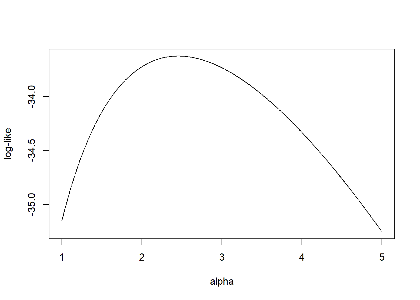
Figure 3.4: Logarithmic Likelihood for a One-Parameter Pareto

We can determine the maximum value of the logarithmic likelihood by taking derivatives and setting it equal to zero. This yields \[ \begin{array}{ll} \frac{ \partial}{\partial \alpha } l(\alpha ) &= 5 \log 500 + 5 / \alpha - \sum_{i=1}^5 \log x_i =_{set} 0 \Rightarrow \\ \hat{\alpha}_{MLE} &= \frac{5}{\sum_{i=1}^5 \log x_i - 5 \log 500 } = 2.453 . \end{array} \]

Naturally, there are many problems where it is not practical to use hand calculations for optimization. Fortunately there are many statistical routines available such as the R function optim.

R Code for Optimization

c1 <- log(521)+log(658)+log(702)+log(819)+log(1217)
nloglike <- function(alpha){-(5*alpha*log(500)+5*log(alpha)-(alpha+1)*c1)}
MLE <- optim(par=1, fn=nloglike)$par

---

This code confirms our hand calculation result where the maximum likelihood estimator is \(\alpha_{MLE} =\) 2.453125.

---

We present a few additional examples to illustrate how actuaries fit a parametric distribution model to a set of claim data using maximum likelihood.

Example 3.5.2. Actuarial Exam Question. Consider a random sample of claim amounts: 8000 10000 12000 15000. You assume that claim amounts follow an inverse exponential distribution, with parameter \(\theta\). Calculate the maximum likelihood estimator for \(\theta\).

Show Example Solution

Solution.

The pdf is \[f_{X}\left( x \right) = \frac{\theta e^{- \frac{\theta}{x}}}{x^{2}}, \] where \(x > 0\).

The likelihood function, \(L\left( \theta \right)\), can be viewed as the probability of the observed data, written as a function of the model’s parameter \(\theta\)

\[ L\left( \theta \right) = \prod_{i = 1}^{4}{f_{X_{i}}\left( x_{i} \right)} = \frac{\theta^{4}e^{- \theta\sum_{i = 1}^{4}\frac{1}{x_{i}}}}{\prod_{i = 1}^{4}x_{i}^{2}}. \]

The log-likelihood function, \(\log L \left( \theta \right)\), is the sum of the individual logarithms

\[ \log L \left( \theta \right) = 4 \log \theta - \theta\sum_{i = 1}^{4}\frac{1}{x_{i}} - 2\sum_{i = 1}^{4}\log x_{i} . \]

Taking a derivative, we have

\[ \frac{d \log L \left( \theta \right)}{d \theta} = \frac{4}{\theta} - \sum_{i = 1}^{4}\frac{1}{x_{i}}. \]

The maximum likelihood estimator of \(\theta\), denoted by \(\hat{\theta}\), is the solution to the equation

\[ \frac{4}{\hat{\theta}} - \sum_{i = 1}^{4}{\frac{1}{x_{i}} = 0}. \]

Thus, \(\hat{\theta} = \frac{4}{\sum_{i = 1}^{4}\frac{1}{x_{i}}} = 10,667.\)

The second derivative of \(\log L \left( \theta \right)\) is given by

\[ \frac{d^{2}\log L\left( \theta \right)}{d\theta^{2}} = \frac{- 4}{\theta^{2}}. \]

Evaluating the second derivative of the loglikelihood function at \(\hat{\theta} = 10,667\) gives a negative value, indicating \(\hat{\theta}\) as the value that maximizes the loglikelihood function.

---

Example 3.5.3. Actuarial Exam Question. A random sample of size 6 is from a lognormal distribution with parameters \(\mu\) and \(\sigma\). The sample values are

\[ 200 \ \ \ 3000 \ \ \ 8000 \ \ \ 60000 \ \ \ 60000 \ \ \ 160000. \]

Calculate the maximum likelihood estimator for \(\mu\) and \(\sigma\).

Show Example Solution

Solution.

The pdf is

\[ f_{X}\left( x \right) = \frac{1}{x \sigma \sqrt{2\pi}}\exp\left( - \frac{1}{2}\left( \frac{\log x - \mu}{\sigma} \right)^{2} \right), \]

where \(x > 0\).

The likelihood function, \(L\left( \mu,\sigma \right)\), is the product of the pdf for each data point.

\[ L\left( \mu,\sigma \right) = \prod_{i = 1}^{6}{f_{X_{i}}\left( x_{i} \right)} = \frac{1}{\sigma^{6}\left( 2\pi \right)^{3}\prod_{i = 1}^{6}x_{i}}\exp\left( - \frac{1}{2}\sum_{i = 1}^{6}\left( \frac{\log x_{i} - \mu}{\sigma} \right)^{2}\right). \]

Taking a logarithm yields the loglikelihood function, \(\log L \left( \mu,\sigma \right)\), which is the sum of the individual logarithms.

\[ \log L\left( \mu,\sigma \right) = - 6 \log \sigma - 3 \log \left( 2\pi \right) - \sum_{i = 1}^{6}\log x_{i} - \frac{1}{2}\sum_{i = 1}^{6}\left( \frac{\log x_{i} - \mu}{\sigma} \right)^{2}. \]

The first partial derivatives are

\[ \begin{array}{ll} \frac{\partial \log L\left( \mu,\sigma \right)}{\partial\mu} &= \frac{1}{\sigma^{2}}\sum_{i = 1}^{6}\left( \log x_{i} - \mu \right) \\ \frac{\partial \log L\left( \mu,\sigma \right)}{\partial\sigma} &= \frac{- 6}{\sigma} + \frac{1}{\sigma^{3}}\sum_{i = 1}^{6}\left( \log x_{i} - \mu \right)^{2}. \end{array} \]

The maximum likelihood estimators of \(\mu\) and \(\sigma\), denoted by \(\hat{\mu}\) and \(\hat{\sigma}\), are the solutions to the equations

\[ \begin{array}{ll} \frac{1}{{\hat{\sigma}}^{2}}\sum_{i = 1}^{6}\left( \log x_{i} - \hat{\mu} \right) &= 0 \\ \frac{- 6}{\hat{\sigma}} + \frac{1}{{\hat{\sigma}}^{3}}\sum_{i = 1}^{6}\left( \log x_{i} - \hat{\mu} \right)^{2} &= 0 . \end{array} \]

These yield the estimates

\[ \hat{\mu} = \frac{\sum_{i = 1}^{6}{\log x_{i}}}{6} = 9.38 \ \ \ \text{and} \ \ \ {\hat{\sigma}}^{2} = \frac{\sum_{i = 1}^{6}\left( \log x_{i} - \hat{\mu} \right)^{2}}{6} = 5.12 . \]

To check that these estimates maximize, and do not minimize, the likelihood, you may also wish to compute the second partial derivatives. These are

\[ \frac{\partial^{2}\log L\left( \mu,\sigma \right)}{\partial\mu^{2}} = \frac{- 6}{\sigma^{2}}, \ \ \ \ \frac{\partial^{2}\log L\left( \mu,\sigma \right)}{\partial\mu\partial\sigma} = \frac{- 2}{\sigma^{3}}\sum_{i = 1}^{6}\left( \log x_{i} - \mu \right) \]

and

\[ \frac{\partial^{2}\log L\left( \mu,\sigma \right)}{\partial\sigma^{2}} = \frac{6}{\sigma^{2}} - \frac{3}{\sigma^{4}}\sum_{i = 1}^{6}\left( \log x_{i} - \mu \right)^{2} . \]

---

Two follow-up questions rely on large sample properties that you may have seen in an earlier course. Appendix Chapter 17 reviews the definition of the likelihood function, introduces its properties, reviews the maximum likelihood estimators, extends their large-sample properties to the case where there are multiple parameters in the model, and reviews statistical inference based on maximum likelihood estimators. In the solutions of these examples we derive the asymptotic variance of maximum-likelihood estimators of the model parameters. We use the delta method to derive the asymptotic variances of functions of these parameters.

Example 3.5.2 - Follow - Up. Refer to Example 3.5.2.

1. Approximate the variance of the maximum likelihood estimator.
2. Determine an approximate 95% confidence interval for \(\theta\).
3. Determine an approximate 95% confidence interval for \(\Pr \left( X \leq 9,000 \right).\)

Show Example Solution

Solution.

a. Taking reciprocal of negative expectation of the second derivative of \(\log L \left( \theta \right)\), we obtain an estimate of the variance of \(\hat{\theta}\), \(\widehat{Var}\left( \hat{\theta} \right) = \left. \ \left\lbrack E\left( \frac{d^{2}\log L \left( \theta \right)}{d\theta^{2}} \right) \right\rbrack^{- 1} \right|_{\theta = \hat{\theta}} = \frac{{\hat{\theta}}^{2}}{4} = 28,446,222\).

It should be noted that as the sample size \(n \rightarrow \infty\), the distribution of the maximum likelihood estimator \(\hat{\theta}\) converges to a normal distribution with mean \(\theta\) and variance \(\hat{V}\left( \hat{\theta} \right)\). The approximate confidence interval in this example is based on the assumption of normality, despite the small sample size, only for the purpose of illustration.

b. The 95% confidence interval for \(\theta\) is given by

\[ 10,667 \pm 1.96\sqrt{28,446,222} = \left( 213.34,\ 21120.66 \right). \]

c. The distribution function of \(X\) is \(F\left( x \right) = 1 - e^{- \frac{x}{\theta}}\). Then, the maximum likelihood estimate of \(g_{\Theta}(\theta) = F\left( 9,000 \right)\) is

\[ g\left( \hat{\theta} \right) = 1 - e^{- \frac{9,000}{10,667}} = 0.57. \]

We use the delta method to approximate the variance of \(g\left( \hat{\theta} \right)\). \[\frac{\text{dg}\left( \theta \right)}{d \theta} = {- \frac{9000}{\theta^{2}}e}^{- \frac{9000}{\theta}}.\]

\(\widehat{Var}\left\lbrack g\left( \hat{\theta} \right) \right\rbrack = \left( - {\frac{9000}{{\hat{\theta}}^{2}}e}^{- \frac{9000}{\hat{\theta}}} \right)^{2}\hat{V}\left( \hat{\theta} \right) = 0.0329\).

The 95% confidence interval for \(F\left( 9000 \right)\) is given by \[ 0.57 \pm 1.96\sqrt{0.0329} = \left( 0.214,\ 0.926 \right). \]

---

Example 3.5.3 - Follow - Up. Refer to Example 3.5.3.

1. Estimate the covariance matrixMatrix where the (i,j)^th element represents the covariance between the ith and jth random variables of the maximum likelihood estimator.
2. Determine approximate 95% confidence intervals for \(\mu\) and \(\sigma\).
3. Determine an approximate 95% confidence interval for the mean of the lognormal distribution.

Show Example Solution

a. To derive the covariance matrix of the mleMaximum likelihood estimate we need to find the expectations of the second derivatives. Since the random variable \(X\) is from a lognormal distribution with parameters \(\mu\) and \(\sigma\), then \(\log X\) is normally distributed with mean \(\mu\) and variance \(\sigma^{2}\).

\[ \mathrm{E}\left( \frac{\partial^{2}\text{log L}\left( \mu,\sigma \right)}{\partial\mu^{2}} \right) = \mathrm{E}\left( \frac{- 6}{\sigma^{2}} \right) = \frac{- 6}{\sigma^{2}} , \]

\[ \mathrm{E}\left( \frac{\partial^{2}\text{log L}\left( \mu,\sigma \right)}{\partial\mu\partial\sigma} \right) = \frac{- 2}{\sigma^{3}}\sum_{i = 1}^{6}{\mathrm{E}\left( \log x_{i} - \mu \right)} = \frac{- 2}{\sigma^{3}}\sum_{i = 1}^{6}\left\lbrack \mathrm{E}\left( \log x_{i} \right) - \mu \right\rbrack = \frac{- 2}{\sigma^{3}}\sum_{i = 1}^{6}\left( \mu - \mu \right) = 0, \]

and

\[ \mathrm{E}\left( \frac{\partial^{2}\text{log L}\left( \mu,\sigma \right)}{\partial\sigma^{2}} \right) = \frac{6}{\sigma^{2}} - \frac{3}{\sigma^{4}}\sum_{i = 1}^{6}{\mathrm{E}\left( \log x_{i} - \mu \right)}^{2} = \frac{6}{\sigma^{2}} - \frac{3}{\sigma^{4}}\sum_{i = 1}^{6}{\mathrm{Var}\left( \log x_{i} \right) = \frac{6}{\sigma^{2}} - \frac{3}{\sigma^{4}}\sum_{i = 1}^{6}{\sigma^{2} = \frac{- 12}{\sigma^{2}}}} . \]

Using the negatives of these expectations we obtain the Fisher information matrix

\[ \begin{bmatrix} \frac{6}{\sigma^{2}} & 0 \\ 0 & \frac{12}{\sigma^{2}} \\ \end{bmatrix}. \]

The covariance matrix, \(\Sigma\), is the inverse of the Fisher information matrix

\[ \Sigma = \begin{bmatrix} \frac{\sigma^{2}}{6} & 0 \\ 0 & \frac{\sigma^{2}}{12} \\ \end{bmatrix}. \]

The estimated matrix is given by

\[ \hat{\Sigma} = \begin{bmatrix} 0.8533 & 0 \\ 0 & 0.4267 \\ \end{bmatrix}. \]

b. The 95% confidence interval for \(\mu\) is given by \(9.38 \pm 1.96\sqrt{0.8533} = \left( 7.57,\ 11.19 \right)\).

The 95% confidence interval for \(\sigma^{2}\) is given by \(5.12 \pm 1.96\sqrt{0.4267} = \left( 3.84,\ 6.40 \right)\).

c. The mean of X is \(\exp\left( \mu + \frac{\sigma^{2}}{2} \right)\). Then, the maximum likelihood estimate of

\[ g\left( \mu,\sigma \right) = \exp\left( \mu + \frac{\sigma^{2}}{2} \right) \]

is

\[ g\left( \hat{\mu},\hat{\sigma} \right) = \exp\left( \hat{\mu} + \frac{{\hat{\sigma}}^{2}}{2} \right) = 153,277. \]

We use the delta method to approximate the variance of the mle \(g\left( \hat{\mu},\hat{\sigma} \right)\).

\(\frac{\partial g\left( \mu,\sigma \right)}{\partial\mu} = \exp\left( \mu + \frac{\sigma^{2}}{2} \right)\) and \(\frac{\partial g\left( \mu,\sigma \right)}{\partial\sigma} = \sigma \exp\left( \mu + \frac{\sigma^{2}}{2} \right)\).

Using the delta method, the approximate variance of \(g\left( \hat{\mu},\hat{\sigma} \right)\) is given by

\[ \left. \ \widehat{Var}\left( g\left( \hat{\mu},\hat{\sigma} \right) \right) = \begin{bmatrix} \frac{\partial g\left( \mu,\sigma \right)}{\partial\mu} & \frac{\partial g\left( \mu,\sigma \right)}{\partial\sigma} \\ \end{bmatrix}\Sigma\begin{bmatrix} \frac{\partial g\left( \mu,\sigma \right)}{\partial\mu} \\ \frac{\partial g\left( \mu,\sigma \right)}{\partial\sigma} \\ \end{bmatrix} \right|_{\mu = \hat{\mu},\sigma = \hat{\sigma}} \\ = \begin{bmatrix} 153,277 & 346,826 \\ \end{bmatrix}\begin{bmatrix} 0.8533 & 0 \\ 0 & 0.4267 \\ \end{bmatrix}\begin{bmatrix} 153,277 \\ 346,826 \\ \end{bmatrix} \\ = 71,374,380,000 . \]

The 95% confidence interval for \(\exp\left( \mu + \frac{\sigma^{2}}{2} \right)\) is given by

\[ 153277 \pm 1.96\sqrt{71,374,380,000} = \left( - 370356,\ 676910 \right). \]

Since the mean of the lognormal distribution cannot be negative, we should replace the negative lower limit in the previous interval by a zero.

---

Example 3.5.4. Wisconsin Property Fund. To see how maximum likelihood estimators work with real data, we return to the 2010 claims data introduced in Section 1.3.

The following snippet of code shows how to fit the exponential, gamma, Pareto, lognormal, and \(GB2\) models. For consistency, the code employs the R package VGAM. The acronym stands for Vector Generalized Linear and Additive Models; as suggested by the name, this package can do far more than fit these models although it suffices for our purposes. The one exception is the \(GB2\) density which is not widely used outside of insurance applications; however, we can code this density and compute maximum likelihood estimators using the optim general purpose optimizer.

Show Example Solution

library(VGAM)
claim_lev <- read.csv("Data/CLAIMLEVEL.csv", header = TRUE) 
claim_data <- subset(claim_lev, Year == 2010); 

# Inference assuming a GB2 Distribution - this is more complicated
# The likelihood function of GB2 distribution (negative for optimization)
lik_gb2 <- function (param) {
  a_1 <- param[1]
  a_2 <- param[2]
  mu <- param[3]
  sigma <- param[4]
  yt <- (log(claim_data$Claim) - mu) / sigma
  logexpyt <- ifelse(yt > 23, yt, log(1 + exp(yt)))
  logdens <- a_1 * yt - log(sigma) - log(beta(a_1,a_2)) - 
    (a_1+a_2) * logexpyt - log(claim_data$Claim) 
  return(-sum(logdens))
}
# "optim" is a general purpose minimization function
gb2_bop <- optim(c(1, 1, 0, 1), lik_gb2, method = c("L-BFGS-B"), 
                 lower = c(0.01, 0.01, -500, 0.01), 
                 upper = c(500, 500, 500, 500), hessian = TRUE)
# Nonparametric Plot
plot(density(log(claim_data$Claim)), main = "", xlab = "Log Expenditures",
     ylim = c(0 ,0.37))
x <- seq(0, 15, by = 0.01)
#Exponential
fit.exp <- vglm(Claim ~ 1, exponential, data = claim_data)
theta = 1 / exp(coef(fit.exp))
fexp_ex <- dgamma(exp(x), scale = exp(-coef(fit.exp)), shape = 1) * exp(x)
lines(x, fexp_ex, col = "red", lty =2)
# Inference assuming a gamma distribution
fit.gamma <- vglm(Claim ~ 1, family = gamma2, data = claim_data)
theta <- exp(coef(fit.gamma)[1]) / exp(coef(fit.gamma)[2])  # theta = mu / alpha
alpha <- exp(coef(fit.gamma)[2]) 
fgamma_ex <- dgamma(exp(x), shape = alpha, scale = theta) * exp(x)
lines(x, fgamma_ex, col = "blue", lty =3)
#Pareto
fit.pareto <- vglm(Claim ~ 1, paretoII, loc = 0, data = claim_data)
fpareto_ex <- dparetoII(exp(x), loc = 0, shape = exp(coef(fit.pareto)[2]), 
                        scale = exp(coef(fit.pareto)[1])) * exp(x)
lines(x, fpareto_ex, col = "purple")
# Lognormal
fit.LN <- vglm(Claim ~ 1, family = lognormal, data = claim_data)
flnorm_ex <- dlnorm(exp(x), mean = coef(fit.LN)[1],
                    sd = exp(coef(fit.LN)[2])) * exp(x)
lines(x, flnorm_ex, col = "lightblue")
# Density for GB II
gb2_density <- function (x) {
  a_1 <- gb2_bop$par[1]
  a_2 <- gb2_bop$par[2]
  mu <- gb2_bop$par[3]
  sigma <- gb2_bop$par[4]
  xt <- (log(x) - mu) / sigma
  logexpxt <- ifelse (xt > 23, yt, log(1 + exp(xt)))
  logdens <- a_1 * xt - log(sigma) - log(beta(a_1, a_2)) - 
    (a_1+a_2) * logexpxt -log(x) 
  exp(logdens)
  }
fGB2_ex = gb2_density(exp(x)) * exp(x)
lines(x, fGB2_ex, col="green")
legend("topleft", c("log(Expend)", "Exponential", "Gamma", "Pareto", 
                    "Lognormal", "GB2"), cex=0.8,
       lty = c(4,2,3,1,1,1), #4 is "longdash"
       col = c("black","red","blue","purple","lightblue","green"))

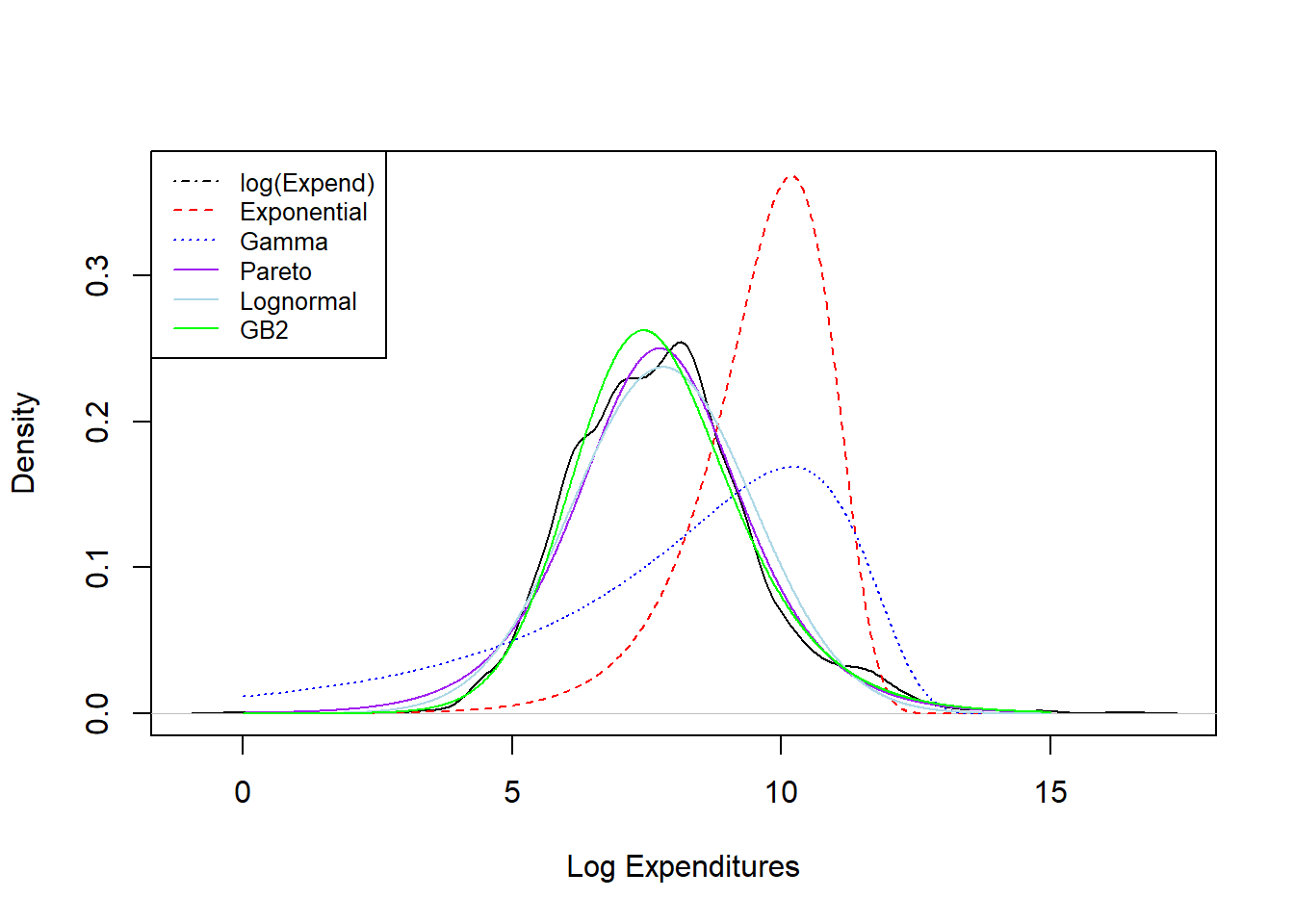
Figure 3.5: Density Comparisons for the Wisconsin Property Fund

Results from the fitting exercise are summarized in Figure 3.5. Here, the black “longdash” curve is a smoothed histogram of the actual data (that we will introduce in Section 4.1); the other curves are parametric curves where the parameters are computed via maximum likelihood. We see poor fits in the red dashed line from the exponential distribution fit and the blue dotted line from the gamma distribution fit. Fits of the other curves, Pareto, lognormal, and GB2, all seem to provide reasonably good fits to the actual data. Chapter 4 describes in more detail the principles of model selection.

---

3.5.2 Maximum Likelihood Estimators using Modified Data

In many applications, actuaries and other analysts wish to estimate model parameters based on individual data that are not limited. However, there are also important applications when only limited, or modified, data are available. This section introduces maximum likelihood estimation for grouped, censored, and truncated data. Later, we will follow up with additional details in Section 4.3.

3.5.2.1 Maximum Likelihood Estimators for Grouped Data

In the previous section we considered the maximum likelihood estimation of continuous models from complete (individual) data. Each individual observation is recorded, and its contribution to the likelihood function is the density at that value. In this section we consider the problem of obtaining maximum likelihood estimates of parameters from grouped dataData bucketed into categories with ranges, such as for use in histograms or frequency tables. The observations are only available in grouped form, and the contribution of each observation to the likelihood function is the probability of falling in a specific group (interval). Let \(n_{j}\) represent the number of observations in the interval \(\left( \left. \ c_{j - 1},c_{j} \right\rbrack \right.\ \) The grouped data likelihood function is thus given by

\[ L\left( \theta \right) = \prod_{j = 1}^{k}\left\lbrack F_X\left( \left. \ c_{j} \right|\theta \right) - F_X\left( \left. \ c_{j - 1} \right|\theta \right) \right\rbrack^{n_{j}}, \]

where \(c_{0}\) is the smallest possible observation (often set to zero) and \(c_{k}\) is the largest possible observation (often set to infinity).

Example 3.5.5. Actuarial Exam Question. For a group of policies, you are given that losses follow the distribution function \(F_X\left( x \right) = 1 - \frac{\theta}{x}\), for \(\theta < x < \infty.\) Further, a sample of 20 losses resulted in the following:

\[ {\small \begin{matrix}\hline \text{Interval} & \text{Number of Losses} \\ \hline (\theta, 10] & 9 \\ (10, 25] & 6 \\ (25, \infty) & 5 \\ \hline \end{matrix} } \]

Calculate the maximum likelihood estimate of \(\theta\).

Show Example Solution

Solution.

The contribution of each of the 9 observations in the first interval to the likelihood function is the probability of \(X \leq 10\); that is, \(\Pr\left( X \leq 10 \right) = F_X\left( 10 \right)\). Similarly, the contributions of each of 6 and 5 observations in the second and third intervals are \(\Pr\left( 10 < X \leq 25 \right) = F_X\left( 25 \right) - F_X(10)\) and \(P\left( X > 25 \right) = 1 - F_X(25)\), respectively. The likelihood function is thus given by \[ \begin{array}{ll} L\left( \theta \right) & = \left\lbrack F_X\left( 10 \right) \right\rbrack^{9}\left\lbrack F_X\left( 25 \right) - F_X(10) \right\rbrack^{6}\left\lbrack 1 - F_X(25) \right\rbrack^{5} \\ & = {\left( 1 - \frac{\theta}{10} \right)}^{9}\left( \frac{\theta}{10} - \frac{\theta}{25} \right)^{6}\left( \frac{\theta}{25} \right)^{5} \\ & = {\left( \frac{10 - \theta}{10} \right)}^{9}\left( \frac{15\theta}{250} \right)^{6}\left( \frac{\theta}{25} \right)^{5}. \end{array} \]

Taking logarithms, the logarithmic likelihood is

\[ \begin{array}{ll} \log L \left( \theta \right) &= 9\log \left( 10 - \theta \right) + 6\log \theta + 5\log \theta - 9\log 10 + 6\log 15 - 6\log 250 - 5\log 25 \\ &= 9\log \left( 10 - \theta \right) + 11\log \theta + constant . \end{array} \]

Here, \(constant\) is a number that does not depend on \(\theta\). Taking derivatives, we have

\[ \frac{d \log L \left( \theta \right)}{d \theta} = \frac{- 9}{\left( 10 - \theta \right)} + \frac{11}{\theta} . \] The maximum likelihood estimator, \(\hat{\theta}\), is the solution to the equation \[ \frac{- 9}{\left( 10 - \hat{\theta} \right)} + \frac{11}{\hat{\theta}} = 0 \] which yields \(\hat{\theta} = 5.5\).

---

3.5.2.2 Maximum Likelihood Estimators for Censored Data

Another possible distinguishing feature of a data gathering mechanism is censoring. While for some events of interest (losses, claims, lifetimes, etc.) the complete dataData where each individual observation is known, and no values are censored, truncated, or grouped maybe available, for others only partial information is available; all that may be known is that the observation exceeds a specific value. The limited policy introduced in Section 3.4.2 is an example of right censoring. Any loss greater than or equal to the policy limit is recorded at the limit. The contribution of the censored observation to the likelihood function is the probability of the random variable exceeding this specific limit. Note that contributions of both complete and censored data share the survival function, for a complete point this survival function is multiplied by the hazard function, but for a censored observation it is not. The likelihood function for censored data is then given by

\[ L(\theta) = \left[ \prod_{i=1}^r f_X(x_i) \right] \left[ S_X(u) \right]^m , \] where \(r\) is the number of known loss amounts below the limit \(u\) and \(m\) is the number of loss amounts larger than the limit \(u\).

Example 3.5.6. Actuarial Exam Question. The random variable \(X\) has survival function: \[ S_{X}\left( x \right) = \frac{\theta^{4}}{\left( \theta^{2} + x^{2} \right)^{2}}. \] Two values of \(X\) are observed to be 2 and 4. One other value exceeds 4. Calculate the maximum likelihood estimate of \(\theta\).

Show Example Solution

Solution.

The contributions of the two observations 2 and 4 are \(f_{X}\left( 2 \right)\) and \(f_{X}\left( 4 \right)\) respectively. The contribution of the third observation, which is only known to exceed 4 is \(S_{X}\left( 4 \right)\). The likelihood function is thus given by \[ L\left( \theta \right) = f_{X}\left( 2 \right)f_{X}\left( 4 \right)S_{X}\left( 4 \right). \] The pdf of \(X\) is given by \[ f_{X}\left( x \right) = \frac{4x\theta^{4}}{\left( \theta^{2} + x^{2} \right)^{3}}. \] Thus, \[ L\left( \theta \right) = \frac{8\theta^{4}}{\left( \theta^{2} + 4 \right)^{3}}\frac{16\theta^{4}}{\left( \theta^{2} + 16 \right)^{3}}\frac{\theta^{4}}{\left( \theta^{2} + 16 \right)^{2}} \\ = \frac{128\theta^{12}}{\left( \theta^{2} + 4 \right)^{3}\left( \theta^{2} + 16 \right)^{5}}, \]

So, \[ \log L\left( \theta \right) = \log 128 + 12\log \theta - 3\log \left( \theta^{2} + 4 \right) - 5\log \left( \theta^{2} + 16 \right) , \]

and

\(\frac{d \log L\left( \theta \right)}{d \theta} = \frac{12}{\theta} - \frac{6\theta}{\left( \theta^{2} + 4 \right)} - \frac{10\theta}{\left( \theta^{2} + 16 \right)}\).

The maximum likelihood estimator, \(\hat{\theta}\), is the solution to the equation \[ \frac{12}{\hat{\theta}} - \frac{6\hat{\theta}}{\left( {\hat{\theta}}^{2} + 4 \right)} - \frac{10\hat{\theta}}{\left( {\hat{\theta}}^{2} + 16 \right)} = 0 \] or \[12\left( {\hat{\theta}}^{2} + 4 \right)\left( {\hat{\theta}}^{2} + 16 \right) - 6{\hat{\theta}}^{2}\left( {\hat{\theta}}^{2} + 16 \right) - 10{\hat{\theta}}^{2}\left( {\hat{\theta}}^{2} + 4 \right) = \\ - 4{\hat{\theta}}^{4} + 104{\hat{\theta}}^{2} + 768 = 0,\] which yields \({\hat{\theta}}^{2} = 32\) and \(\hat{\theta} = 5.7\).

---

3.5.2.3 Maximum Likelihood Estimators for Truncated Data

This section is concerned with the maximum likelihood estimation of the continuous distribution of the random variable \(X\) when the data is incomplete due to truncation. If the values of \(X\) are truncated at \(d\), then it should be noted that we would not have been aware of the existence of these values had they not exceeded \(d\). The policy deductible introduced in Section 3.4.1 is an example of left truncation. Any loss less than or equal to the deductible is not recorded. The contribution to the likelihood function of an observation \(x\) truncated at \(d\) will be a conditional probability and the \(f_{X}\left( x \right)\) will be replaced by \(\frac{f_{X}\left( x \right)}{S_{X}\left( d \right)}\). The likelihood function for truncated data is then given by

\[ L(\theta) = \prod_{i=1}^k \frac{f_X(x_i)}{S_X(d)} , \] where \(k\) is the number of loss amounts larger than the deductible \(d\).

Example 3.5.7. Actuarial Exam Question. For the single-parameter Pareto distribution with \(\theta = 2\), maximum likelihood estimation is applied to estimate the parameter \(\alpha\). Find the estimated mean of the ground up loss distribution based on the maximum likelihood estimate of \(\alpha\) for the following data set:

• Ordinary policy deductible of 5, maximum covered loss of 25 (policy limit 20)
• 8 insurance payment amounts: 2, 4, 5, 5, 8, 10, 12, 15
• 2 limit payments: 20, 20.

Show Example Solution

Solution.

The contributions of the different observations can be summarized as follows:

• For the exact loss: \(f_{X}\left( x \right)\)
• For censored observations: \(S_{X}\left( 25 \right)\).
• For truncated observations: \(\frac{f_{X}\left( x \right)}{S_{X}\left( 5 \right)}\).

Given that ground up losses smaller than 5 are omitted from the data set, the contribution of all observations should be conditional on exceeding 5. The likelihood function becomes

\[ L\left( \alpha \right) = \frac{\prod_{i = 1}^{8}{f_{X}\left( x_{i} \right)}}{\left\lbrack S_{X}\left( 5 \right) \right\rbrack^{8}}\left\lbrack \frac{S_{X}\left( 25 \right)}{S_{X}\left( 5 \right)} \right\rbrack^{2}. \]

For the single-parameter Pareto the probability density and distribution functions are given by

\[ f_{X}\left( x \right) = \frac{\alpha\theta^{\alpha}}{x^{\alpha + 1}} \ \ \text{and} \ \ F_{X}\left( x \right) = 1 - \left( \frac{\theta}{x} \right)^{\alpha}, \] for \(x > \theta\), respectively. Then, the likelihood is given by \[ L\left( \alpha \right) = \frac{\alpha^{8}}{\prod_{i = 1}^{8}x_{i}^{\alpha + 1}}\frac{5^{10\alpha}}{25^{2\alpha}} . \]

Taking logarithms, the loglikelihood function is

\[ \log L \left( \alpha \right) = 8\log\alpha - \left( \alpha + 1 \right)\sum_{i = 1}^{8}{\log x_{i}} + 10\alpha \log 5 - 2\alpha \log 25. \]

Taking a derivative, we have

\[ \frac{d \log L \left( \alpha \right)}{d \theta} = \frac{8}{\alpha} - \sum_{i = 1}^{8}{\log x_{i}} + 10\log 5 - 2\log 25. \]

With this, the maximum likelihood estimator, \(\hat{\alpha}\), is the solution to the equation

\[ \frac{8}{\hat{\alpha}} - \sum_{i = 1}^{8}{\log x_{i}} + 10\log 5 - 2\log 25 = 0, \] which yields \[ \begin{array}{ll} \hat{\alpha} &= \frac{8}{\sum_{i = 1}^{8}{\log x_{i}} - 10\log 5 + 2\log 25} \\ &= \frac{8}{(\log 7 + \log 9 + \cdots + \log 20) - 10\log 5 + 2\log 25} = 0.785. \end{array} \] The mean of the single-parameter Pareto is finite for \(\alpha > 1\) (see Appendix Section 18.2). Since \(\hat{\alpha} = 0.785 < 1\). Then, the mean is infinite.

---

Show Quiz Solution

---

3.6 Further Resources and Contributors

Contributors

• Zeinab Amin, The American University in Cairo, is the principal author of this chapter. Email: zeinabha@aucegypt.edu for chapter comments and suggested improvements.
• Many helpful comments have been provided by Hirokazu (Iwahiro) Iwasawa, iwahiro@bb.mbn.or.jp .
• Other chapter reviewers include: Rob Erhardt, Samuel Kolins, Tatjana Miljkovic, Michelle Xia, and Jorge Yslas.

Exercises

Here are a set of exercises that guide the viewer through some of the theoretical foundations of Loss Data Analytics. Each tutorial is based on one or more questions from the professional actuarial examinations – typically the Society of Actuaries Exam C/STAM.

Severity Distribution Guided Tutorials

Further Readings and References

Notable contributions include: Cummins and Derrig (2012), Frees and Valdez (2008), Klugman, Panjer, and Willmot (2012), Kreer et al. (2015), McDonald (1984), McDonald and Xu (1995), Tevet (2016), and Venter (1983).

Bibliography

Cummins, J. David, and Richard A. Derrig. 2012. Managing the Insolvency Risk of Insurance Companies: Proceedings of the Second International Conference on Insurance Solvency. Vol. 12. Springer Science & Business Media.

Frees, Edward W., and Emiliano A. Valdez. 1998. “Understanding Relationships Using Copulas.” North American Actuarial Journal 2 (01): 1–25.

2008. “Hierarchical Insurance Claims Modeling.” Journal of the American Statistical Association 103 (484): 1457–69.

Klugman, Stuart A., Harry H. Panjer, and Gordon E. Willmot. 2012. Loss Models: From Data to Decisions. John Wiley & Sons.

Kreer, Markus, Ayşe Kızılersü, Anthony W Thomas, and Alfredo D Egı́dio dos Reis. 2015. “Goodness-of-Fit Tests and Applications for Left-Truncated Weibull Distributions to Non-Life Insurance.” European Actuarial Journal 5 (1): 139–63.

McDonald, James B. 1984. “Some Generalized Functions for the Size Distribution of Income.” Econometrica: Journal of the Econometric Society, 647–63.

McDonald, James B, and Yexiao J Xu. 1995. “A Generalization of the Beta Distribution with Applications.” Journal of Econometrics 66 (1-2): 133–52.

Tevet, Dan. 2016. “Applying Generalized Linear Models to Insurance Data.” Predictive Modeling Applications in Actuarial Science: Volume 2, Case Studies in Insurance, 39.

Venter, Gary. 1983. “Transformed Beta and Gamma Distributions and Aggregate Losses.” In Proceedings of the Casualty Actuarial Society, 70:289–308. 133 & 134.