Chapter 5 Aggregate Loss Models

Chapter Preview. This chapter introduces probability models for describing the aggregate (total) claims that arise from a portfolio of insurance contracts. We present two standard modeling approaches, the individual risk model and the collective risk model. Further, we discuss strategies for computing the distribution of the aggregate claims, including exact methods for special cases, recursion, and simulation. Finally, we examine the effects of individual policy modifications such as deductibles, coinsurance, and inflation, on the frequency and severity distributions, and thus on the aggregate loss distribution.

5.1 Introduction

The objective of this chapter is to build a probability model to describe the aggregate claims by an insurance system occurring in a fixed time period. The insurance system could be a single policy, a group insurance contract, a business line, or an entire book of an insurer’s business. In this chapter, aggregate claimsThe sum of all claims observed in a period of time refer to either the number or the amount of claims from a portfolio of insurance contracts. However, the modeling framework can be readily applied in the more general setup.

Consider an insurance portfolio of \(n\) individual contracts, and let \(S\) denote the aggregate losses of the portfolio in a given time period. There are two approaches to modeling the aggregate losses \(S\), the individual risk model and the collective risk model. The individual risk modelA modeling approach for aggregate losses in which the loss from each individual contract is considered. emphasizes the loss from each individual contract and represents the aggregate losses as:

\[ S_n=X_1 +X_2 +\cdots+X_n, \]

where \(X_i~(i=1,\ldots,n)\) is interpreted as the loss amount from the \(i\)th contract. It is worth stressing that \(n\) denotes the number of contracts in the portfolio and thus is a fixed number rather than a random variable. For the individual risk model, one usually assumes the \(X_{i}\)’s are independent. Because of different contract features such as coverageInsurance coverage is the amount of risk or liability that is covered for an individual or entity by an insurance policy. and exposureA measure of the rating units for which rates are applied to determine the premium. for example, exposures may be measured on a per unit basis (e.g. a family with auto insurance under one contract may have an exposure of 2 cars) or per $1,000 of value (e.g. homeowners insurance)., the \(X_{i}\)’s are not necessarily identically distributed. A notable feature of the distribution of each \(X_i\) is the probability mass at zero corresponding to the event of no claims.

The collective risk modelA modeling approach for aggregate losses in which the aggregate loss is represented in terms of a frequency distribution and a severity distribution. represents the aggregate losses in terms of a frequency distribution and a severity distribution:

\[ S_N=X_1 +X_2 + \cdots + X_N . \]

Here, one thinks of a random number of claims \(N\) that may represent either the number of losses or the number of payments. In contrast, in the individual risk model, we use a fixed number of contracts \(n\). We think of \(X_1, X_2, \ldots, X_N\) as representing the amount of each loss. Each loss may or may not correspond to a unique contract. For instance, there may be multiple claims arising from a single contract. It is natural to think about \(X_i>0\) because if \(X_i=0\) then no claim has occurred. Typically we assume that conditional on \(N=n\), \(X_{1},X_{2},\ldots ,X_{n}\) are iidIndependent and identically distributed random variables. The distribution of \(N\) is known as the frequency distributionThe random number of claims that occur under the collective risk model., and the common distribution of \(X\) is known as the severity distributionThe randomly distributed amount of each loss under the collective risk model.. We further assume \(N\) and \(X\) are independent. With the collective risk model, we may decompose the aggregate losses into the frequency (\(N\)) process and the severity (\(X\)) model. This flexibility allows the analyst to comment on these two separate components. For example, sales growth due to lower underwriting standards could lead to higher frequency of losses but might not affect severity. Similarly, inflationInflation is a sustained increase in the general price level of goods and services over a period of time. or other economic forces could have an impact on severity but not on frequency.

Show Quiz Solution

---

5.2 Individual Risk Model

As noted earlier, for the individual risk model, we think of \(X_i\) as the loss from \(i\)th contract and interpret

\[ S_n=X_1 +X_2 +\cdots+X_n , \]

to be the aggregate loss from all contracts in a portfolio or group of contracts. Here, the \(X_i\)’s are not necessarily identically distributed and we have \[ {\rm E}(S_n) = \sum_{i=1}^{n} {\rm E}(X_i)~. \]

Under the independence assumption on \(X_i\)’s (which implies \(\mathrm{Cov}\left( X_i, X_j \right) = 0\) for all \(i \neq j\)), it can further be shown that

\[ \begin{aligned} {\rm Var}(S_n) &= \sum_{i=1}^{n} {\rm Var}(X_i) \\ P_{S_n}(z) &= \prod_{i=1}^{n}P_{X_i}(z) \\ M_{S_n}(t) &= \prod_{i=1}^{n}M_{X_i}(t), \end{aligned} \]

where \(P_{S_n}(\cdot)\) and \(M_{S_n}(\cdot)\) are the probability generating function (pgf) and the moment generating function (mgf) of \(S_n\), respectively. The distribution of each \(X_i\) contains a probability mass at zero, corresponding to the event of no claims from the \(i\)th contract. One strategy to incorporate the zero mass in the distribution is to use the two-part framework: \[\begin{aligned} X_i = I_i\times B_i = \left\{\begin{array}{ll} 0~, & \text{if }~ I_i=0 \\ B_i~, & \text{if }~ I_i=1 . \end{array} \right. \end{aligned}\] Here, \(I_i\) is a Bernoulli variable indicating whether or not a loss occurs for the \(i\)th contract, and \(B_i\) is a random variable with nonnegative supportThe set of all outcomes for a random variable following some distribution. for example, exponentially distributed random variable x has support x>0. representing the amount of losses of the contract given loss occurrence. Assume that \(I_1 ,\ldots,I_n ,B_1 ,\ldots,B_n\) are mutually independent. Denote \({\rm Pr} (I_i =1)=q_i\), \(\mu_i={\rm E}(B_i)\), and \(\sigma_i^2={\rm Var}(B_i)\). It can be shown (see Technical Supplement 5.A.1 for details) that \[\begin{aligned} \mathrm{E}(S_n)& =\sum_{i=1}^n ~q_i ~\mu _i \\ \mathrm{Var}(S_n) & =\sum_{i=1}^n \left( q_i \sigma _i^2+q_i (1-q_i)\mu_i^2 \right)\\ P_{S_n}(z) & =\prod_{i=1}^n \left( 1-q_i+q_i P_{B_i}(z) \right)\\ M_{S_n}(t) & =\prod_{i=1}^n \left( 1-q_i+q_i M_{B_i}(t) \right) . \end{aligned}\] A special case of the above model is when \(B_i\) follows a degenerate distribution with \(\mu_i=b_i\) and \(\sigma^2_i=0\). One example is term life insuranceA term life insurance policy is payable only if death of the insured occurs within a specified time, such as 5 or 10 years, or before a specified age. or a pure endowmentA pure endowment is an insurance policy that is payable at the end of the policy period if the insured is still alive. if the insured has died, there is nothing paid in the form of benefits. insurance where \(b_i\) represents the insurance benefit amount of the \(i\)th contract.

Another strategy to accommodate the zero mass in the loss from each contract is to consider them in aggregate at the portfolio level, as in the collective risk model. Here, the aggregate loss is \(S_{N} = X_1 + \cdots + X_N\), where \(N\) is a random variable representing the number of non-zero claims that occurred out of the entire group of contracts. Thus, not every contract in the portfolio may be represented in this sum, and \(S_N=0\) when \(N=0\). The collective risk model will be discussed in detail in the next section.

---

Example 5.2.1. Actuarial Exam Question. An insurance company sold 300 fire insurance policies as follows:

\[ {\small \begin{matrix} \begin{array}{c c c} \hline \text{Number of} & \text{Policy} & \text{Probability of}\\ \text{Policies} & \text{Maximum} & \text{Claim Per Policy}\\ & (M_i) & (q_i) \\ \hline 100 & 400 & 0.05\\ 200 & 300 & 0.06\\ \hline \end{array} \end{matrix} } \]

You are given:
(i) The claim amount for each policy, \(X_i\), is uniformly distributed between \(0\) and the policy maximum \(M_i\).
(ii) The probability of more than one claim per policy is \(0\).
(iii) Claim occurrences are independent.

Calculate the mean, \(\mathrm{E~}(S_{300})\), and variance, \(\mathrm{Var~}(S_{300})\), of the aggregate claims. How would these results change if every claim is equal to the policy maximum?

Show Example Solution

Solution. The aggregate claims are \(S_{300} = X_1+\cdots+X_{300}\), where \(X_1, \ldots, X_{300}\) are independent but not identically distributed. Policy claims amounts are uniformly distributed on \((0,M_i)\), so the mean claim amount is \(M_i/2\) and the variance is \(M_i^2/12\). Thus, for policy \(i=1,\ldots,300\), we have \[ {\small \begin{matrix} \begin{array}{ccccc} \hline \text{Number of} & \text{Policy} & \text{Probability of} & \text{Mean} & \text{Variance}\\ \text{Policies} & \text{Maximum} & \text{Claim Per Policy} & \text{Amount} & \text{Amount}\\ & (M_i) & (q_{i}) & (\mu_{i}) & (\sigma_{i}^2) \\ \hline 100 & 400 & 0.05 & 200 & 400^2/12\\ 200 & 300 & 0.06 & 150 & 300^2/12 \\ \hline \end{array} \end{matrix} } \]

The mean of the aggregate claims is \[\mathrm{E~} (S_{300}) = \sum_{i=1}^{300} q_i \mu_i = 100\left\{0.05(200)\right\} + 200\left\{0.06 (150) \right\} = 2,800\]

The variance of the aggregate claims is

\[ \begin{array}{ll} \mathrm{Var~}(S_{300}) &= \sum_{i=1}^{300} \left( q_i \sigma _i^2+q_i (1-q_i)\mu_i^2 \right) ~~~~ \text{since } X_i \text{'s are independent} \\ &= 100\left\{ 0.05 \left(\frac{400^2}{12}\right) +0.05 (1-0.05 )200^2 \right\} \\ & \ \ \ \ + 200\left\{ 0.06 \left(\frac{300^2}{12}\right) +0.06 (1-0.06 )150^2 \right\}\\ &= 600,467. \end{array} \]

---

Follow-Up. Now suppose everybody receives the policy maximum \(M_i\) if a claim occurs. What is the expected aggregate loss \(\mathrm{E~}(\tilde{S})\) and variance of the aggregate loss \(\mathrm{Var~}(\tilde{S})\)?

Each policy claim amount \(X_i\) is now deterministic and fixed at \(M_i\) instead of a randomly distributed amount, so \(\sigma_i^2 = \mathrm{Var~} (X_i) = 0\) and \(\mu_i = M_i\). Again, the probability of a claim occurring for each policy is \(q_i\). Under these circumstances, the expected aggregate loss is \[\begin{aligned} \mathrm{E~}(\tilde{S}) &= \sum_{i=1}^{300} q_i \mu_i = 100 \left\{0.05(400) \right\} + 200 \left\{ 0.06(300) \right\} = 5,600 . \end{aligned}\]

The variance of the aggregate loss is \[ \begin{aligned} \mathrm{Var~}(\tilde{S}) &= \sum_{i=1}^{300} \left( q_i \sigma _i^2+q_i (1-q_i )\mu_i^2 \right) = \sum_{i=1}^{300} \left( q_i (1-q_i) \mu_i^2 \right) \\ &= 100 \left\{(0.05) (1-0.05) 400^2\right\} + 200 \left\{(0.06) (1-0.06)300^2\right\} \\ &= 1,775,200 . \end{aligned} \]

---

The individual risk model can also be used for claim frequency. If \(X_i\) denotes the number of claims from the \(i\)th contract, then \(S_n\) is interpreted as the total number of claims from the portfolio. In this case, the above two-part framework still applies since there is a probability mass at zero for contracts that do not experience any claims. Assume \(X_i\) belongs to the \((a,b,0)\) class with pmfProbability mass function denoted by \(p_{ik} = \Pr(X_i=k)\) for \(k=0,1,\ldots\) (see Section 2.3). Let \(X_i^{T}\) denote the associated zero-truncated distribution in the \((a,b,1)\) class with pmf \(p_{ik}^T=p_{ik}/(1-p_{i0})\) for \(k=1,2,\ldots\) (see Section 2.5.1). Using the relationship between their probability generating functions (see Technical Supplement 5.A.2 for details): \[\begin{aligned} P_{X_i}(z) = p_{i0} +(1-p_{i0}) P_{X_i^{T}}(z), \end{aligned}\] we can write \(X_i=I_i\times B_i\) with \(q_i={\rm Pr}(I_i=1)={\rm Pr}(X_i>0)=1-p_{i0}\) and \(B_i=X_i^T\). Notice that in this case, we have a zero-modified distribution since the \(I_i\) variable covers the modified probability mass at zero with \(q_i = \Pr(I_i=1)\), while the \(B_i=X_i^T\) covers the discrete non-zero frequency portion. See Section 2.5.1 for the relationship between zero-truncated and zero-modified distributions.

---

Example 5.2.2. An insurance company sold a portfolio of 100 independent homeowners insurance policies, each of which has claim frequency following a zero-modified Poisson distribution, as follows:

\[ {\small \begin{matrix} \begin{array}{cccc} \hline \text{Type of} & \text{Number of} & \text{Probability of} & \lambda \\ \text{Policy} & \text{Policies} & \text{At Least 1 Claim} & \\ \hline \text{Low-risk} & 40 & 0.03 & 1 \\ \text{High-risk} & 60 & 0.05 & 2 \\ \hline \end{array} \end{matrix} } \] Find the expected value and variance of the claim frequency for the entire portfolio.

Show Example Solution

Solution. For each policy, we can write the zero-modified Poisson claim frequency \(N_i\) as \(N_i = I_i \times B_i\), where \[q_i = \Pr(I_i = 1) = \Pr(N_i > 0) = 1-p_{i0} .\] For the low-risk policies, we have \(q_i = 0.03\) and for the high-risk policies, we have \(q_i=0.05\). Further, \(B_i = N_i^T\), the zero-truncated version of \(N_i\). Thus, we have

\[ \begin{aligned} \mu_i &={\rm E}(B_i) = {\rm E}(N_i^T) = \frac{\lambda}{1-e^{-\lambda}} \\ \sigma_i^2 &={\rm Var}(B_i) = {\rm Var}(N_i^T) = \frac{\lambda [1-(\lambda+1)e^{-\lambda}]}{(1-e^{-\lambda})^2} . \end{aligned} \]

Using \(n=100\), let the portfolio claim frequency be \(S_{100} = \sum_{i=1}^{100} N_i\). Using the formulas above, the expected claim frequency of the portfolio is

\[ \begin{aligned} \mathrm{E~} (S_{100}) &= \sum_{i=1}^{100} q_i \mu_i \\ & = 40\left[0.03 \left(\frac{1}{1-e^{-1}} \right) \right] + 60 \left[0.05 \left( \frac{2}{1-e^{-2}} \right) \right] \\ &= 40(0.03)(1.5820) + 60(0.05)(2.3130) = 8.8375 . \end{aligned} \]

The variance of the claim frequency of the portfolio is

\[ \begin{aligned} \mathrm{Var~}(S_{100}) &= \sum_{i=1}^{100} \left( q_i \sigma _i^2+q_i (1-q_i )\mu_i^2 \right) \\ &= 40 \left[ 0.03 \left(\frac{1-2e^{-1}}{(1-e^{-1})^2} \right) + 0.03(0.97)(1.5820^2) \right] \\ & \ \ \ + 60 \left[0.05 \left( \frac{2[1-3e^{-2}]}{ (1-e^{-2})^2} \right) + 0.05(0.95)(2.3130^2) \right] \\ &= 23.7214 . \end{aligned} \] Note that equivalently, we could have calculated the mean and variance of an individual policy directly using the relationship between the zero-modified and zero-truncated Poisson distributions (see Section 2.3).

---

To understand the distribution of the aggregate loss, one could use the central limit theoremGiven certain conditions, the arithmetic mean of a large number of replications of independent random variables, each with a finite mean and variance, will be approximately normally distributed, regardless of the underlying distribution. to approximate the distribution of \(S_n\) for large \(n\). Denote \(\mu_{S_n}={\rm E}(S_n)\) and \(\sigma^2_{S_n}={\rm Var}(S_n)\) and let \(Z\sim N(0,1)\), a standard normal random variable with cdfCumulative distribution function \(\Phi\). Then the cdf of \(S_n\) can be approximated as follows: \[\begin{aligned} F_{S_n}(s) &= {\rm Pr}({S_n}\leq s) = \Pr \left( \frac{S_n - \mu_{S_n}}{\sigma_{S_n}} \leq \frac{s-\mu_{S_n}}{\sigma_{S_n}} \right) \\ &\approx \Pr\left( Z \leq \frac{s-\mu_{S_n}}{\sigma_{S_n}} \right) = \Phi \left(\frac{s-\mu_{S_n}}{\sigma_{S_n}}\right) . \end{aligned}\]

---

Example 5.2.3. Actuarial Exam Question - Follow-Up. As in the Example 5.2.1 earlier, an insurance company sold 300 fire insurance policies, with claim amounts \(X_i\) uniformly distributed between 0 and the policy maximum \(M_i\). Using the normal approximation, calculate the probability that the aggregate claim amount \(S_{300}\) exceeds \(\$3,500\).

Show Example Solution

Solution. We have seen earlier that \(\mathrm{E}(S_{300})=2,800\) and \(\mathrm{Var}(S_{300}) = 600,467\). Then \[\begin{aligned} {\rm Pr}(S_{300} > 3,500) &= 1 - {\rm Pr}(S_{300} \leq 3,500) \\ &\approx 1- \Phi \left( \frac{3,500-2,800}{\sqrt{600,467}} \right) = 1 - \Phi \left( 0.90334 \right) \\ &= 1 - 0.8168 = 0.1832 . \end{aligned}\]

---

For small \(n\), the distribution of \(S_n\) is likely skewed, and the normal approximation would be a poor choice. To examine the aggregate loss distribution, we go back to first principles. Specifically, the distribution can be derived recursively. Define \(S_k=X_1 + \cdots + X_k, k=1,\ldots,n\).

For \(k=1\): \[F_{S_1}(s) = {\rm Pr}(S_1\leq s) = {\rm Pr}(X_1\leq s) = F_{X_1}(s).\] For \(k=2,\ldots,n\): \[\begin{aligned} F_{S_k}(s)&={\Pr}(X_1+\cdots+X_k\leq s) ={\Pr}(S_{k-1}+X_k\leq s) \\ &={\rm E}_{X_k}\left[{\rm Pr}(S_{k-1}\leq s-X_k|X_k)\right]= {\rm E}_{X_k}\left[F_{S_{k-1}}(s-X_k)\right] . \end{aligned}\]

A special case is when \(X_i\)’s are identically distributed. Let \(F_X(x)={\Pr}(X\leq x)\) be the common distribution of \(X_i, ~i=1,\ldots,n\). We define \[F^{*n}_X(x)={\Pr}(X_1+\cdots+X_n\leq x) ,\] the \(n\)-fold convolutionThe convolution of probability distributions is the distribution corresponding to the addition of independent random variables. of \(F_X\). More generally, we can compute \(F_X^{\ast n}\) recursively. Begin the recursion at \(k=1\) using \(F_X^{\ast 1} \left(x \right) =F_X(x)\). Next, for \(k=2\), we have

\[\begin{eqnarray*} F_X^{\ast 2} \left(x \right) &=& \Pr(X_1 + X_2 \le x) = \mathrm{E}_{X_2} \left[ \Pr(X_1 \le x - X_2|X_2) \right] \\ &=& \mathrm{E}_{X_2} \left[ F(x - X_2) \right] \\ &=&\left\{\begin{array}{ll} \int_{0}^{x} F(x-y) f(y) dy & \text{for continuous } X_i \text{'s} \\ \sum_{y \le x} F(x-y) f(y) & \text{for discrete } X_i \text{'s} \\ \end{array}\right. \end{eqnarray*}\]

Recall \(F(0) = 0\).

Similarly for \(k=n\), we have \(S_n = X_1 + X_2 + \cdots + X_n\) and

\[\begin{eqnarray*} F^{\ast n}\left(x\right) &=& \Pr(S_n \le x) = \Pr(S_{n-1} + X_n \le x)\\ &=&\mathrm{E}_{X_n} \left[ \Pr(S_{n-1} \le x - X_n|X_n) \right] \\ &=&\mathrm{E}_X \left[ F^{\ast(n-1)}(x - X) \right] \\ &=& \left\{\begin{array}{ll} \int_{0}^{x} F^{\ast(n-1)}(x-y)f(y)dy & \text{for continuous } X_i \text{'s} \\ \sum_{y \le x} F^{\ast(n-1)}(x-y)f(y) & \text{for discrete } X_i \text{'s} \\ \end{array}\right. \end{eqnarray*}\]

When the \(X_i\)’s are independent and belong to the same family of distributions, there are some simple cases where \(S_n\) has a closed form. This makes it easy to compute \(\Pr(S_n \le x)\). This property is known as closed under convolution, meaning the distribution of the sum of independent random variables belongs to the same family of distributions as that of the component variables, just with different parameters. Table 5.1 provides a few examples.

Table 5.1. Closed Form Partial Sum Distributions

\[ {\small \begin{matrix} \begin{array}{l|l|l} \hline \text{Distribution of } X_i & \text{Abbreviation} & \text{Distribution of } S_n \\ \hline \text{Normal with mean } \mu_i \text{ and variance } \sigma_i^2 & N(\mu_i,\sigma_i^2) & N\left(\sum_{i=1}^{n}\mu_i,~\sum_{i=1}^{n}\sigma_i^2\right) \\ \text{Exponential with mean } \theta & Exp(\theta) & Gam(n,\theta)\\ \text{Gamma with shape } \alpha_i \text{ and scale } \theta & Gam(\alpha_i,\theta) & Gam\left(\sum_{i=1}^n\alpha_i,\theta\right) \\ \text{Poisson with mean (and variance) } \lambda_i & Poi(\lambda_i)& Poi\left(\sum_{i=1}^{n}\lambda_i\right)\\ \text{Binomial with } m_i \text{ trials and } q \text{ success probability} & Bin(m_i, q)& Bin\left(\sum_{i=1}^n m_i, q\right)\\ \text{Geometric with mean } \beta & Geo(\beta) & NB(\beta,n)\\ \text{Negative binomial with mean } r_i \beta~& NB(\beta,r_i)& NB\left(\beta,\sum_{i=1}^n r_i\right)\\ ~ ~ ~ \text{ and variance } ~r_i \beta (1+\beta) & & \\ \hline \end{array} \end{matrix} } \]

---

Example 5.2.4. Gamma Distribution. Assume that \(X_1,\ldots,X_n\) are independent random variables with \(X_i \sim Gam(\alpha_i, \theta)\). The mgf of \(X_i\) is \(M_{X_i}(t) = (1 - \theta t)^{- \alpha_i}\). Thus, the mgf of the sum \(S_n = X_1 + \cdots + X_n\) is \[\begin{aligned} M_{S_n}(t) &= \prod_{i=1}^n M_{X_i}(t) ~~~~ \text{from the independence of } X_i \text{'s} \\ &= \prod_{i=1}^n (1 - \theta t)^{- \alpha_i} = (1-\theta t)^{-\sum_{i=1}^n \alpha_i }~ , \end{aligned}\]

which is the mgf of a gamma random variable with parameters \((\sum_{i=1}^n \alpha_i, \theta)\). Thus, \(S_n \sim Gam(\sum_{i=1}^n \alpha_i, \theta)\).

---

Example 5.2.5. Negative Binomial Distribution. Assume that \(X_1,\ldots, X_n\) are independent random variables with \(X_i \sim NB(\beta, r_i)\). The pgf of \(X_i\) is \(P_{X_i}(z) = \left[1-\beta(z-1) \right]^{-r_i}\). Thus, the pgf of the sum \(S_n =X_1+\cdots+X_n\) is

\[ \begin{aligned} P_{S_n}(z) &= \mathrm{E~}\left[ z^{S_n} \right] \\ &= \mathrm{E~}\left[z^{X_1}\right] \cdots \mathrm{E~}\left[z^{X_n}\right] ~~~~ \text{from the independence of } X_i \text{'s} \\ &= \prod_{i=1}^n P_{X_i}(z) = \prod_{i=1}^n \left[1-\beta(z-1) \right]^{-r_i} = \left[1-\beta(z-1) \right]^{-\sum_{i=1}^n r_i} ~, \end{aligned} \]

which is the pgf of a negative binomial random variable with parameters \((\beta, \sum_{i=1}^n r_i)\). Thus, \(S_n \sim NB(\beta, \sum_{i=1}^n r_i)\).

---

Example 5.2.6. Actuarial Exam Question (modified). The annual number of doctor visits for each individual in a family of 4 has geometric distribution with mean 1.5. The annual numbers of visits for the family members are mutually independent. An insurance pays 100 per doctor visit beginning with the 4th visit per family. Calculate the probability that the family will not receive an insurance payment this year.

Show Example Solution

Solution. Let \(X_i \sim Geo(\beta=1.5)\) be the number of doctor visits for one individual in the family and \(S_4 = X_1 + X_2 + X_3 + X_4\) be the number of doctor visits for the family. The sum of 4 independent geometric random variables each with mean \(\beta=1.5\) follows a negative binomial distribution, i.e. \(S_4 \sim NB(\beta=1.5, r=4)\).

If the insurance pays 100 per visit beginning with the 4th visit for the family, then the family will not receive an insurance payment if they have less than 4 claims. This probability is \[\begin{aligned} \Pr(S_4 < 4) &= \Pr(S_4 = 0) + \Pr(S_4 = 1) + \Pr(S_4 = 2) +\Pr(S_4 = 3) \\ &= (1+1.5)^{-4} + \frac{4(1.5)}{(1+1.5)^5} + \frac{4(5)(1.5^2)}{2(1+1.5)^6} + \frac{4(5)(6)(1.5^3)}{3!(1+1.5)^7}\\ &= 0.0256 + 0.0614 + 0.0922 + 0.1106 = 0.2898 . \end{aligned}\]

---

Show Quiz Solution

---

5.3 Collective Risk Model

5.3.1 Moments and Distribution

Under the collective risk model \(S_N=X_1+\cdots+X_N\), \(\{X_i\}\) are iid, and independent of \(N\). Let \(\mu = {\rm E}\left( X_{i}\right)\) and \(\sigma ^{2} = {\rm Var}\left(X_{i}\right)\) for all \(i\). Thus, conditional on \(N\), we have that the expectation of the sum is the sum of expectations and that the variance of the sum is the sum of variances,

\[ \begin{aligned} {\rm E}(S|N) &= {\rm E}(X_1 + \cdots + X_N|N) = \mu N \\ {\rm Var}(S|N) &= {\rm Var}(X_1 + \cdots + X_N|N) = \sigma^2 N . \end{aligned} \]

Using the law of iterated expectationsA decomposition of the expected value of a random variable into conditional components. specifically, for random variables x and y, e(x) = e[e(x|y)]. from Appendix Section 16.2, the mean of the aggregate loss is \[ {\rm E}(S_N)={\rm E}_N[{\rm E}_S(S|N)] = {\rm E}_N(N\mu) = \mu ~{\rm E}(N). \]

Using the law of total varianceA decomposition of the variance of a random variable into conditional components. specifically, for random variables x and y on the same probability space, var(x) = e[var(y|x)] + var[e(x|y)]. from Appendix Section 16.2, the variance of the aggregate loss is

\[ \begin{aligned} {\rm Var}(S_N) &= {\rm E}_N[{\rm Var}(S_N|N)] + {\rm Var}_N[{\rm E}(S_N|N)] \\ &= \mathrm{E}_N \left[ \sigma^2 N \right] + \mathrm{Var}_N\left[ \mu N \right] \\ &=\sigma^2~{\rm E}[N] + \mu^2~ {\rm Var}[N] . \end{aligned} \]

Special Case: Poisson Distributed Frequency. If \(N \sim Poi (\lambda)\), then \[\begin{aligned} \mathrm{E}(N) &= \mathrm{Var}(N) = \lambda\\ \mathrm{E}(S_N) &= \lambda ~\mathrm{E}(X)\\ \mathrm{Var}(S_N) &= \lambda (\sigma^2 + \mu^2) = \lambda ~\mathrm{E} (X^2) . \end{aligned}\]

---

Example 5.3.1. Actuarial Exam Question. The number of accidents follows a Poisson distribution with mean 12. Each accident generates 1, 2, or 3 claimants with probabilities 1/2, 1/3, and 1/6 respectively.

Calculate the variance in the total number of claimants.

Show Example Solution

Solution. \[\begin{aligned} & \mathrm{E}(X^2) = 1^2 \left( \frac{1}{2}\right) + 2^2\left(\frac{1}{3} \right) + 3^2\left(\frac{1}{6}\right) = \frac{10}{3} \\ \Rightarrow &\mathrm{Var}(S_N) = \lambda \ \mathrm{E}(X^2) = 12\left(\frac{10}{3}\right) = 40 . \end{aligned}\]

Alternatively, using the general approach, \(\mathrm{Var}(S_N) = \sigma^2 \mathrm{E}(N) + \mu^2 \mathrm{Var}(N)\), where

\[ \begin{aligned} \mathrm{E}(N) &= \mathrm{Var}(N) = 12 \\ \mu &= \mathrm{E}(X) = 1\left(\frac{1}{2}\right) + 2\left(\frac{1}{3}\right) + 3\left(\frac{1}{6}\right) = \frac{5}{3} \\ \sigma^2 &= \mathrm{E}(X^2) - [\mathrm{E}(X)]^2 = \frac{10}{3} - \frac{25}{9} = \frac{5}{9} \\ \Rightarrow \ \mathrm{Var}(S_N) &= \left(\frac{5}{9}\right)\left(12\right) + \left(\frac{5}{3}\right)^2\left(12\right) = 40 . \end{aligned} \]

---

In general, the moments of \(S_N\) can be derived from its moment generating function (mgf). Because \(X_i\)’s are iid, we denote the mgf of \(X\) as \(M_{X}(t) = \mathrm{E~}(e^{tX})\). Using the law of iterated expectations, the mgf of \(S_N\) is

\[\begin{aligned} M_{S_N}(t) &= \mathrm{E}(e^{t S_N})=\mathrm{E}_N[~\mathrm{E}(e^{tS_N}|N)~]\\ &= \mathrm{E}_N \left[ ~\mathrm{E}\left( e^{t(X_1+\cdots+X_N)}\right) ~\right] = \mathrm{E}_N \left[ \mathrm{E}(e^{tX_1})\cdots\mathrm{E}(e^{tX_N}) \right] ~~~~ \text{since } X_i \text{'s are independent} \\ &= \mathrm{E}_N[~(M_{X}(t))^N~] . \end{aligned}\]

Now, recall that the probability generating function (pgf) of \(N\) is \(P_N(z) = \mathrm{E}(z^N)\). Denote \(M_{X}(t)=z\). Substituting into the expression for the mgf of \(S_N\) above, it is shown

\[\begin{aligned} M_{S_N}(t) = \mathrm{E~}(z^N) = P_{N}(z) = P_{N}[M_{X}(t)]. \end{aligned}\]

Similarly, if \(S_N\) is discrete, one can show the pgf of \(S_N\) is: \[\begin{aligned} P_{S_N}(z) = P_{N}[P_{X}(z)] . \end{aligned}\]

To get \(\mathrm{E}(S_N) = M_{S_N}'(0)\), we use the chain rule \[ M_{S_N}'(t) = \frac{\partial}{\partial t} P_{N}(M_{X}(t)) = P_{N}'(M_{X}(t)) M_{X}'(t)\\ \] and recall \(M_{X}(0) = 1, M_{X}'(0) = \mathrm{E}(X) = \mu, P_{N}'(1) = \mathrm{E}(N)\). So, \[\begin{aligned} \mathrm{E}(S_N) = M_{S_N}'(0) = P_{N}'(M_{X}(0)) M_{X}'(0) = \mu {\rm E}(N) . \end{aligned}\]

Similarly, one could use relation \(\mathrm{E}(S_N^2) = M_{S_N}''(0)\) to get \[\mathrm{Var}(S_N) = \sigma^2 \mathrm{E}(N) + \mu^2 \mathrm{Var}(N).\]

Special Case. Poisson Frequency. Let \(N \sim Poi (\lambda)\). Thus, the pgf of \(N\) is \(P_N (z) = e^{\lambda(z-1)}\) and the mgf of \(S_N\) is \[\begin{aligned} M_{S_N}(t) &= P_N[M_X(t)] = e^{\lambda(M_{X}(t) - 1)}. \end{aligned}\]

Taking derivatives yields \[\begin{aligned} M_{S_N}'(t) &= e^{\lambda(M_{X}(t) - 1)}~ \lambda~ M_{X}'(t) = M_{S_N}(t) ~\lambda ~M_{X}'(t)\\ M_{S_N}''(t) &= M_{S_N}(t) ~\lambda~ M_{X}''(t) + [~M_{S_N}(t)~\lambda~ M_{X}'(t)~] ~\lambda~ M_{X}'(t) . \end{aligned}\]

Evaluating these at \(t=0\) yields \[\begin{aligned} \mathrm{E}(S_N) &= M_{S_N}'(0) = \lambda \mathrm{E}(X) = \lambda \mu \end{aligned}\] and

\[\begin{aligned} M_{S_N}''(0) &= \lambda \mathrm{E}(X^2) + \lambda^2 \mu^2\\ \Rightarrow \mathrm{Var}(S_N) &= \lambda \mathrm{E}(X^2) + \lambda^2 \mu^2 - (\lambda \mu)^2 = \lambda~ \mathrm{E}(X^2). \end{aligned}\]

---

Example 5.3.2. Actuarial Exam Question. You are the producer of a television quiz show that gives cash prizes. The number of prizes, \(N\), and prize amount, \(X\), have the following distributions:

\[ {\small \begin{matrix} \begin{array}{ccccc}\hline n & \Pr(N=n) & & x & \Pr(X=x)\\ \hline 1 & 0.8 & & 0 & 0.2 \\ 2 & 0.2 & & 100 & 0.7 \\ & & & 1000 & 0.1\\\hline \end{array} \end{matrix} } \]

Your budget for prizes equals the expected aggregate cash prizes plus the standard deviation of aggregate cash prizes. Calculate your budget.

Show Example Solution

Solution. We need to calculate the mean and standard deviation of the aggregate (sum) of cash prizes. The moments of the frequency distribution \(N\) are \[\begin{aligned} \mathrm{E}(N) &= 1 (0.8) + 2 (0.2) =1.2\\ \mathrm{E}(N^2) &= 1^2 (0.8) + 2^2 (0.2) =1.6\\ \mathrm{Var}(N) &= \mathrm{E}(N^2) - \left[ \mathrm{E}(N) \right]^2= 0.16 . \end{aligned}\]

The moments of the severity distribution \(X\) are \[\begin{aligned} \mathrm{E}(X) &= 0 (0.2) + 100 (0.7) + 1000 (0.1) = 170 = \mu\\ \mathrm{E}(X^2) &= 0^2 (0.2) + 100^2 (0.7) + 1000^2 (0.1) = 107,000\\ \mathrm{Var}(X) &= \mathrm{E}(X^2) - \left[ \mathrm{E}(X) \right]^2=78,100 = \sigma^2 . \end{aligned}\]

Thus, the mean and variance of the aggregate cash prize are \[\begin{aligned} \mathrm{E}(S_N) &= \mu \mathrm{E}(N) = 170 (1.2) = 204 \\ \mathrm{Var}(S_N) &= \sigma^2 \mathrm{E}(N) + \mu^2 \mathrm{Var}(N)\\ &= 78,100 (1.2) + 170^2 (0.16) = 98,344 . \end{aligned}\]

This gives the following required budget \[\begin{aligned} Budget &= \mathrm{E}(S_N) + \sqrt{\mathrm{Var}(S_N)} \\ &= 204 + \sqrt{98,344} = 517.60 . \end{aligned}\]

---

The distribution of \(S_N\) is called a compound distributionA random variable follows a compound distribution if it is parameterized and contains at least one parameter that is itself a random variable. for example, the tweedie distribution is a compound distribution., and it can be derived based on the convolution of \(F_X\) as follows: \[\begin{aligned} F_{S_N}(s) &= \Pr \left(X_1 + \cdots + X_N \le s \right) \\ &= \mathrm{E} \left[ \Pr \left(X_1 + \cdots + X_N \le s|N=n \right) \right]\\ &= \mathrm{E} \left[ F_{X}^{\ast N}(s) \right] \\ &= p_0 + \sum_{n=1}^{\infty }p_n F_{X}^{\ast n}(s) . \end{aligned}\]

---

Example 5.3.3. Actuarial Exam Question. The number of claims in a period has a geometric distribution with mean \(4\). The amount of each claim \(X\) follows \(\Pr(X=x) = 0.25, \ x=1,2,3,4\), i.e. a discrete uniform distribution on \(\{1,2,3,4\}\). The number of claims and the claim amounts are independent. Let \(S_N\) denote the aggregate claim amount in the period. Calculate \(F_{S_N}(3)\).

Show Example Solution

Solution. By definition, we have \[\begin{aligned} F_{S_N}\left(3 \right) &= {\rm Pr}\left(\sum_{i=1}^N X_i \leq 3\right) = \sum_{n=0}^\infty {\rm Pr}\left(\sum_{i=1}^n X_i\leq 3|N=n\right){\rm Pr}(N=n) \\ &= \sum_n F^{\ast n} \left(3 \right) p_n = \sum_{n=0}^3 F^{\ast n}(3) p_n \\ &= p_0 + F^{\ast 1}(3) \ p_1 + F^{\ast 2}(3) \ p_2 + F^{\ast 3}(3) \ p_3 . \end{aligned}\] Because \(N \sim Geo(\beta=4)\), we know that \[\begin{aligned} p_n &= \frac{1}{1+\beta} \left(\frac{\beta}{1+ \beta} \right)^n = \frac{1}{5} \left(\frac{4}{5} \right)^n . \end{aligned}\] For the claim severity distribution, recursively, we have \[\begin{aligned} F^{\ast 1}(3) &= \Pr(X \le 3) = \frac{3}{4} \\ F^{\ast 2}(3) &= \sum_{y \le 3} F^{\ast 1} (3-y) f(y) = F^{\ast 1}(2)f(1) + F^{\ast 1}(1)f(2) \\ &= \frac{1}{4}\left[F^{\ast 1} (2) + F^{\ast 1}(1)\right] = \frac{1}{4}\left[{\rm Pr}(X\leq 2) + {\rm Pr}(X \leq 1) \right] \\ &= \frac{1}{4} \left(\frac{2}{4} + \frac{1}{4} \right) = \frac{3}{16}\\ F^{\ast 3}(3) &= \Pr(X_1+X_2 + X_3 \le 3) = \Pr(X_1=X_2=X_3=1) = \left(\frac{1}{4} \right)^3 . \end{aligned}\] Notice that we did not need to recursively calculate \(F^{\ast 3}(3)\) by recognizing that each \(X \in \{1,2,3,4\}\), so the only way of obtaining \(X_1+X_2+X_3 \leq 3\) is to have \(X_1=X_2=X_3=1\). Additionally, for \(n \geq 4\), \(F^{\ast n} (3)=0\) since it is impossible for the sum of 4 or more \(X\)’s to be less than 3. For \(n=0\), \(F^{\ast 0}(3) = 1\) since the sum of 0 \(X\)’s is 0, which is always less than 3. Laying out the probabilities systematically,

\[\begin {matrix} \begin{array}{c c c c}\hline x & F^{\ast 1}(x) & F^{\ast 2}(x) & F^{\ast 3}(x)\\ \hline 0 & & & \\ 1 & \frac{1}{4} & 0 & \\ 2 & \frac{2}{4} & \left( \frac{1}{4} \right)^2 & \\ 3 & \frac{3}{4} & \frac{3}{16} & \left( \frac{1}{4} \right)^3 \\ \hline \end{array} \end{matrix}\]

Finally, \[\begin{aligned} F_{S_N}(3) &= p_0 + F^{\ast 1}(3) \ p_1 + F^{\ast 2}(3) \ p_2 + F^{\ast 3}(3) \ p_3 \\ &= \frac{1}{5} + \frac{3}{4}\left(\frac{4}{25} \right) + \frac{3}{16} \left( \frac{16}{125} \right) + \frac{1}{64} \left( \frac{64}{625}\right) = 0.3456 .\\ \end{aligned}\]

---

When \(\mathrm{E}(N)\) and \(\mathrm{Var}(N)\) are known, one may also use a type of central limit theorem to approximate the distribution of \(S_N\) as in the individual risk model. That is, \(\frac{S_N - \mathrm{E}(S_N)}{\sqrt{\mathrm{Var}(S_N)}}\) approximately follows the standard normal distribution \(N(0,1)\). From this type of central limit theorem, the approximation works well if \(\mathrm{E}[N]\) is sufficiently large.

---

Example 5.3.4. Actuarial Exam Question. You are given:

\[ {\small \begin{matrix} \begin{array}{ c | c c } \hline & \text{Mean} & \text{Standard Deviation}\\ \hline \text{Number of Claims} & 8 & 3\\ \text{Individual Losses} & 10,000 & 3,937\\ \hline \end{array} \end{matrix} } \] As a benchmark, use the normal approximation to determine the probability that the aggregate loss will exceed 150\(\%\) of the expected loss.

Show Example Solution

Solution. To use the normal approximation, we must first find the mean and variance of the aggregate loss \(S\) \[\begin{aligned} \mathrm{E}(S_N) &= \mu \ \mathrm{E}(N) = 10,000(8) = 80,000\\ \mathrm{Var}(S_N) &= \sigma^2 \ \mathrm{E}(N) + \mu^2 \ \mathrm{Var}(N)\\ &= 3937^2(8) + 10000^2 (3^2) = 1,023,999,752\\ \sqrt{\mathrm{Var}(S_N)} &= 31,999.996 \approx 32,000 . \end{aligned}\]

Then under the normal approximation, aggregate loss \(S_N\) is approximately normal with mean 80,000 and standard deviation 32,000. The probability that \(S_N\) will exceed 150\(\%\) of the expected aggregate loss is therefore \[\begin{aligned} \Pr(S_N>1.5 \mathrm{E}(S_N)~) &= \Pr \left( \frac{S_N - \mathrm{E} (S_N)}{\sqrt{\mathrm{Var}(S_N)}} > \frac{1.5 ~\mathrm{E}(S_N) - \mathrm{E} (S_N)}{\sqrt{\mathrm{Var}(S_N)}} \right) \\ &\approx \Pr \left( Z > \frac{0.5~ \mathrm{E}(S_N)}{\sqrt{\mathrm{Var}(S_N)} } \right), ~~~~ \text{where } Z\sim N(0,1) \\ &= \Pr \left( Z > \frac{0.5(80,000)}{32,000} \right) = \Pr( Z > 1.25) \\ &= 1-\Phi(1.25) = 0.1056 . \end{aligned}\]

---

Example 5.3.5. Actuarial Exam Question. For an individual over \(65\):
(i) The number of pharmacy claims is a Poisson random variable with mean \(25\).
(ii) The amount of each pharmacy claim is uniformly distributed between \(5\) and \(95\).
(iii) The amounts of the claims and the number of claims are mutually independent.
Estimate the probability that aggregate claims for this individual will exceed \(2000\) using the normal approximation.

Show Example Solution

Solution. We have claim frequency \(N \sim Poi(\lambda = 25)\) and claim severity \(X \sim U \left(5, 95 \right)\). To use the normal approximation, we need to find the mean and variance of the aggregate claims \(S_N\). Note

\[\begin{matrix} \begin{array}{lll} \mathrm{E} (N) = 25 & & \mathrm{Var} (N) = 25\\ \mathrm{E}(X) = \frac{5+95}{2} = 50 = \mu & & \mathrm{Var}(X) = \frac{(95-5)^2}{12} = 675 = \sigma^2 .\\ \end{array} \end{matrix}\]

Then for \(S_N\), \[\begin{aligned} \mathrm{E}(S_N) &= \mu \ \mathrm{E} (N) = 50(25) = 1,250\\ \mathrm{Var}(S_N) &= \sigma^2 \ \mathrm{E}(N) + \mu^2 \ \mathrm{Var}(N)\\ &= 675 (25) + 50^2 (25) = 79,375 . \end{aligned}\]

Using the normal approximation, \(S_N\) is approximately normal with mean 1,250 and variance 79,375. The probability that \(S_N\) exceeds 2,000 is \[\begin{aligned} \Pr(S_N>2,000) &= \Pr \left(\frac{S_N - \mathrm{E} (S_N)}{\sqrt{\mathrm{Var} (S_N)}} > \frac{2,000- \mathrm{E} (S_N)}{\sqrt{\mathrm{Var} (S_N)}} \right) \\ &\approx \Pr\left( Z > \frac{2,000-1,250}{\sqrt{79,375}} \right), ~~~~ \text{where } Z\sim N(0,1) \\ &= \Pr (Z > 2.662) = 1-\Phi(2.662) = 0.003884. \end{aligned}\]

---

5.3.2 Stop-loss Insurance

Recall the coverage modifications on the individual policy level in Section 3.4. Insurance on the aggregate loss \(S_N\), subject to a deductibleA deductible is a parameter specified in the contract. typically, losses below the deductible are paid by the policyholder whereas losses in excess of the deductible are the insurer’s responsibility (subject to policy limits and coninsurance). \(d\), is called . The expected value of the amount of the aggregate loss in excess of the deductible,

\[\begin{eqnarray*} \mathrm{E}[(S-d)_+] \end{eqnarray*}\] is known as the net stop-loss premium.

To calculate the net stop-loss premium, we have

\[\begin{eqnarray*} \mathrm{E}(S_N-d)_+ &=& \left\{\begin{array}{ll} \int_{d}^{\infty}(s-d) f_{S_N}(s) ds& \text{for continuous } S_N\\ \sum_{s>d}(s-d) f_{S_N}(s) & \text{for discrete } S_N\\ \end{array}\right.\\ &=& \mathrm{E}(S_N) - \mathrm{E}(S_N\wedge d)\\ \end{eqnarray*}\]

---

Example 5.3.6. Actuarial Exam Question. In a given week, the number of projects that require you to work overtime has a geometric distribution with \(\beta=2\). For each project, the distribution of the number of overtime hours in the week, \(X\), is as follows:

\[ {\small \begin{matrix} \begin{array}{ccc} \hline x & & f(x)\\ \hline 5 & & 0.2 \\ 10 & & 0.3 \\ 20 & & 0.5\\ \hline \end{array} \end{matrix} } \]

The number of projects and the number of overtime hours are independent. You will get paid for overtime hours in excess of 15 hours in the week. Calculate the expected number of overtime hours for which you will get paid in the week.

Show Example Solution

Solution. The number of projects in a week requiring overtime work has distribution \(N \sim Geo(\beta=2)\), while the number of overtime hours worked per project has distribution \(X\) as described above. The aggregate number of overtime hours in a week is \(S_N\) and we are therefore looking for \[\mathrm{E}(S_N-15)_+ = \mathrm{E}(S_N) - \mathrm{E}(S_N \wedge 15).\]

To find \(\mathrm{E}(S_N) = \mathrm{E}(X) ~\mathrm{E}(N)\), we have \[\begin{aligned} &\mathrm{E}(X) = 5(0.2) + 10(0.3)+ 20(0.5)= 14 \\ &\mathrm{E}(N) = 2 \\ \Rightarrow \ &\mathrm{E}(S) = \mathrm{E}(X) ~ \mathrm{E}(N) = 14(2) = 28 . \end{aligned}\]

To find \(\mathrm{E} (S_N \wedge 15) = 0 \Pr (S_N=0) + 5 \Pr(S_N=5) + 10 \Pr(S_N=10) + 15 \Pr(S_N \geq 15)\), we have \[\begin{aligned} \Pr(S_N=0) &= \Pr(N=0) = \frac{1}{1+\beta} = \frac{1}{3} \\ \Pr(S_N=5) &= \Pr(X=5, \ N=1) = 0.2 \left(\frac{2}{9} \right)= \frac{0.4}{9}\\ \Pr(S_N=10) &= \Pr(X=10, \ N=1) + \Pr(X_1=X_2=5, N=2) \\ &= 0.3 \left(\frac{2}{9} \right) + (0.2)(0.2) \left( \frac{4}{27} \right)= 0.0726 \\ \Pr(S_N \geq 15) &= 1 - \left(\frac{1}{3} + \frac{0.4}{9} + 0.0726 \right) = 0.5496\\ \Rightarrow \mathrm{E}(S_N \wedge 15) &= 0 \Pr (S_N=0) + 5 \Pr(S_N=5) + 10 \Pr(S_N=10) + 15 \Pr(S_N \geq 15) \\ &= 0 \left( \frac{1}{3} \right) + 5 \left( \frac{0.4}{9} \right) + 10 (0.0726) + 15 (0.5496) = 9.193 .\\ \end{aligned}\] Therefore, \[\begin{aligned} \mathrm{E}(S_N-15)_+ &= \mathrm{E}(S_N) - \mathrm{E}(S_N \wedge 15) \\ &= 28 - 9.193 = 18.807 . \end{aligned}\]

---

Recursive Net Stop-Loss Premium Calculation. For the discrete case, this can be computed recursively as \[\begin{aligned} \mathrm{E}\left[ \left( S_N-(j+1)h \right) _{+} \right]=\mathrm{E}\left[ ( S_N-jh )_{+} \right] -h \left( 1-F_{S_N}(jh) \right) . \end{aligned}\] This assumes that the support of \(S_N\) is equally spaced over units of \(h\).

To establish this, we assume that \(h=1\). We have \[\begin{aligned} \mathrm{E}\left[ \left( S_N-(j+1) \right) _{+} \right] &=\mathrm{E}(S_N) - \mathrm{E}[S_N\wedge (j+1)] \ ,\ \text{ and } \\ \mathrm{E}\left[ \left( S_N - j \right)_+ \right] &=\mathrm{E}(S_N) - \mathrm{E}[S_N\wedge j] \end{aligned}\]

Thus, \[\begin{aligned} \mathrm{E}\left[ \left(S_N-(j+1) \right) _{+}\right] - \mathrm{E}\left[ ( S_N-j )_{+} \right] &= \left\{\mathrm{E}(S_N) - \mathrm{E}(S_N\wedge (j+1)) \right\} - \left\{\mathrm{E}(S_N) - \mathrm{E}(S_N\wedge j) \right\} \\ &= \mathrm{E}\left(S_N \wedge j \right) - \mathrm{E}\left[ S \wedge (j+1) \right] \end{aligned}\]

We can write \[\begin{aligned} \mathrm{E}\left[S_N\wedge (j+1)\right] &= \sum_{x=0}^{j}xf_{S_N}(x) + (j+1)~\Pr(S_N \ge j+1) \\ &= \sum_{x=0}^{j-1}x f_{S_N}(x) + j~\Pr(S_N=j) + (j+1)~\Pr(S_N \ge j+1) \end{aligned}\]

Similarly, \[\begin{aligned} \mathrm{E}(S_N\wedge j) = \sum_{x=0}^{j-1}xf_{S_N}(x) + j~\Pr(S_N\ge j) \end{aligned}\]

With these expressions, we have

\[ \begin{aligned} & \mathrm{E}\left[ \left( S_N-(j+1) \right) _{+} \right] - \mathrm{E~}\left[ ( S_N-j )_{+} \right] \\ &= \mathrm{E}\left(S_N \wedge j \right) - \mathrm{E}\left[ S \wedge (j+1) \right] \\ &= \left\{ \sum_{x=0}^{j-1}xf_{S_N}(x) + j~\Pr(S_N\ge j) \right\} - \left\{ \sum_{x=0}^{j-1}x f_{S_N}(x) + j~\Pr(S_N=j) + (j+1)~\Pr(S_N \ge j+1) \right\} \\ &= j~\left[\Pr(S_N \geq j) - \Pr(S_N=j) \right]- (j+1)~\Pr(S_N \ge j+1) \\ &= j~\Pr( S_N > j) - (j+1)~\Pr(S_N \ge j+1) ~~~~ \text{ (note } \Pr(S_N > j) = \Pr(S_N \geq j+1) \text{)} \\ &= -\Pr(S_N\ge j+1) = -\left[1 - F_{S_N}(j)\right], \end{aligned} \]

as required.

---

Example 5.3.7. Actuarial Exam Question - Continued. Recall that the goal of this question was to calculate \(\mathrm{E~}(S_N-15)_+\). Note that the support of \(S_N\) is equally spaced over units of 5, so this question can also be done recursively, using the expression above with steps of \(h=5\):

• Step 1:
  \[\begin{aligned} \mathrm{E~}(S_N-5)_+ &= \mathrm{E}(S_N) - 5 [1-\Pr(S_N \leq 0) ]\\ %\Pr (S_N\geq 5) \\ &= 28 - 5 \left(1 - \frac{1}{3}\right) = \frac{74}{3}=24.6667 . \end{aligned}\]

• Step 2:
  \[\begin{aligned} \mathrm{E~}(S_N-10)_+ &= \mathrm{E~}(S_N-5)_+ - 5 [1-\Pr(S_N \leq 5)]\\ %\Pr (S_N\ge 10) \\ &= \frac{74}{3} - 5\left( 1 - \frac{1}{3} - \frac{0.4}{9}\right) = 21.555 . \end{aligned}\]

• Step 3: \[\begin{aligned} \mathrm{E~}(S_N-15)_+ &= \mathrm{E~}(S_N-10)_+ - 5 [1-\Pr(S_N \leq 10)] \\ %\Pr (S_N\ge 15) \\ &= \mathrm{E~}(S_N-10)_+ - 5\Pr (S_N\ge 15) \\ &= 21.555 - 5 (0.5496) = 18.807 . \end{aligned}\]

---

5.3.3 Analytic Results

There are a few combinations of claim frequency and severity distributions that result in an easy-to-compute distribution for aggregate losses. This section provides some simple examples. Although these examples are computationally convenient, they are generally too simple to be used in practice.

---

Example 5.3.8. One has a closed-form expression for the aggregate loss distribution by assuming a geometric frequency distribution and an exponential severity distribution.

Assume that claim count \(N\) is geometric with mean \(\mathrm{E}(N)=\beta\), and that claim amount \(X\) is exponential with \(\mathrm{E}(X)=\theta\). Recall that the pgf of \(N\) and the mgf of \(X\) are: \[\begin{aligned} P_N (z) &=\frac{1}{1- \beta (z-1)}\\ M_{X}(t) &=\frac{1}{1-\theta t} . \end{aligned}\] Thus, the mgf of aggregate loss \(S_N\) can be expressed two ways (for details, see Technical Supplement 5.A.3) \[\begin{eqnarray} M_{S_N}(t) &=& P_N [M_{X}(t)] = \frac{1}{1 - \beta \left( \frac{1}{1-\theta t} - 1\right)} \nonumber\\ &=& 1+ \frac{\beta}{1+\beta} \left([1-\theta(1+\beta)t]^{-1}-1 \right)\\ &=& \frac{1}{1+\beta}(1) +\frac{\beta}{1+\beta} \left( \frac{1}{1-\theta (1+\beta)t}\right) . \end{eqnarray}\]

From (5.1), we note that \(S_N\) is equivalent to the compound distribution of \(S_N=X^{*}_1+\cdots+X^{*}_{N^{*}}\), where \(N^{*}\) is a Bernoulli with mean \(\beta/(1+\beta)\) and \(X^{*}\) is an exponential with mean \(\theta(1+\beta)\). To see this, we examine the mgf of \(S\): \[\begin{aligned} M_{S_N}(t) = P_N [M_{X}(t)] = P_{N^{*}} [M_{X^{*}}(t)], \end{aligned}\] where \[\begin{aligned} P_{N^*} (z) &=1+ \frac{\beta}{1+ \beta} (z-1),\\ M_{X^*} (t) &=\frac{1}{1- {{\theta(1+\beta)}} t}. \end{aligned}\]

From (5.2), we note that \(S_N\) is also equivalent to a two-point mixture of 0 and \(X^{*}\). Specifically,

\[ \begin{array}{cl} S_N &= \left\{ \begin{array}{cl} 0 & {\rm with~ probability ~Pr}(N^*=0) = 1/(1+\beta) \\ Y^{*} & {\rm with~ probability ~Pr}(N^*=1) = \beta/(1+\beta) . \end{array} \right. \end{array} \]

The distribution function of \(S_N\) is: \[\begin{eqnarray*} \Pr(S_N=0) &=& \frac{1}{1+\beta}\\ \Pr(S_N>s) &=& \Pr(X^*>s) =\frac{\beta}{1+\beta} \exp\left( -\frac{s}{ \theta (1+\beta)}\right) \end{eqnarray*}\] with pdfProbability density function for \(s>0\), \[\begin{eqnarray*} f_{S_N}(s) = \frac{\beta}{\theta (1+\beta)^2}\exp\left( -\frac{s}{ \theta (1+\beta)}\right) . \end{eqnarray*}\]

---

Example 5.3.9. Consider a collective risk model with an exponential severity and an arbitrary frequency distribution. Recall that if \(X_i\sim Exp(\theta)\), then the sum of iid exponential random variables, \(S_n=X_1+\cdots+X_n\), has a gamma distribution, i.e. \(S_n\sim Gam(n,\theta)\). This has cdf: \[\begin{eqnarray*} F_{X}^{\ast n}(s) &=& \Pr (S_n \le s) = \int_{0}^{s} \frac{1}{\Gamma(n)\theta^n}s^{n-1}\exp\left(-\frac{s}{\theta}\right) ds\\ &=& 1-\sum_{j=0}^{n-1}\frac{1}{j!}\left( \frac{s}{\theta}\right)^j e^{-s/\theta } . \end{eqnarray*}\] The last equality is derived by applying integration by parts \(n-1\) times.

For the aggregate loss distribution, we can interchange the order of summations in the second line below to get

\[ \begin{array}{ll} F_{S}\left(s\right) &= p_{0}+\sum_{n=1}^{\infty }p_n F_{X}^{\ast n}\left(s\right)\\ &= 1 - \sum_{n=1}^{\infty }p_n \sum_{j=0}^{n-1}\frac{1}{j!} \left( \frac{s}{\theta}\right)^j e^{-s/\theta }\\ &= 1-e^{-s/\theta}\sum_{j=0}^{\infty} \frac{1}{j!} \left( \frac{s}{\theta} \right)^j \overline{P}_j \end{array} \]

where \(\overline{P}_j =p_{j+1}+p_{j+2}+\cdots = \Pr (N>j)\) is the “survival function” of the claims count distribution.

---

5.3.4 Tweedie Distribution

In this section, we examine a particular compound distribution where the number of claims has a Poisson distribution and the amount of claims has a gamma distribution. This specification leads to what is known as a Tweedie distributionA compound distribution that is a poisson sum of gamma random variables. because it can accommodate a discrete probability mass at zero and a continuous positive component, it is suitable for modeling aggregate insurance claims.. The Tweedie distribution has a mass probability at zero and a continuous component for positive values. Because of this feature, it is widely used in insurance claims modeling, where the zero mass is interpreted as no claims and the positive component as the amount of claims.

Specifically, consider the collective risk model \(S_N=X_1+\cdots+X_N\). Suppose that \(N\) has a Poisson distribution with mean \(\lambda\), and each \(X_i\) has a gamma distribution with shape parameterA numerical parameter of a parametric distribution affecting the shape of a distribution rather than simply shifting it (as a location parameter does) or stretching/shrinking it (as a scale parameter does). \(\alpha\) and scale parameterA numerical parameter of a parametric distribution that stretches/shrinks the distribution without changing its location or shape. the larger the scale parameter, the more spread out the distribution. the scale parameter is also the reciprocal of the rate parameter. for example, the normal distribution has scale parameter . \(\gamma\). The Tweedie distribution is derived as the Poisson sum of gamma variables. To understand the distribution of \(S_N\), we first examine the mass probability at zero. The aggregate loss is zero when no claims occurred, i.e. \[{\rm Pr}(S_N=0)= {\rm Pr}(N=0)=e^{-\lambda}.\] In addition, note that \(S_N\) conditional on \(N=n\), denoted by \(S_n=X_1+\cdots+X_n\), follows a gamma distribution with shape \(n\alpha\) and scale \(\gamma\). Thus, for \(s>0\), the density of a Tweedie distribution can be calculated as \[\begin{aligned} f_{S_N}(s)&=\sum_{n=1}^{\infty} p_n f_{S_n}(s)\\ &=\sum_{n=1}^{\infty}e^{-\lambda}\frac{(\lambda)^n}{n!}\frac{\gamma^{na}}{\Gamma(n\alpha)}s^{n\alpha-1}e^{-s\gamma} . \end{aligned}\] Thus, the Tweedie distribution can be thought of a mixture of zero and a positive valued distribution, which makes it a convenient tool for modeling insurance claims and for calculating pure premiums. The mean and variance of the Tweedie compound Poisson model are: \[{\rm E} (S_N)=\lambda\frac{\alpha}{\gamma}~~~~{\rm and}~~~~{\rm Var} (S_N)=\lambda\frac{\alpha(1+\alpha)}{\gamma^2}.\]

As another important feature, the Tweedie distribution is a special case of exponential dispersionA set of distributions that represents a generalisation of the natural exponential family and also plays an important role in generalized linear models. models, a class of models used to describe the random component in generalized linear modelsCommonly known by the acronym glm. an extension of the linear regression model where the dependent variable is a member of the linear exponential family. glm encompasses linear, binary, count, and long-tailed, regressions all as special cases.. To see this, we consider the following reparameterization: \[\begin{equation*} \lambda=\frac{\mu^{2-p}}{\phi(2-p)},~~~~\alpha=\frac{2-p}{p-1},~~~~\frac{1}{\gamma}=\phi(p-1)\mu^{p-1} . \end{equation*}\] With the above relationships, one can show that the distribution of \(S_N\) is

\[ f_{S_N}(s)=\exp\left[\frac{1}{\phi}\left(\frac{-s}{(p-1)\mu^{p-1}}-\frac{\mu^{2-p}}{2-p}\right)+C(s;\phi)\right] \]

where

\[ C(s;\phi)=\left\{\begin{array}{ll} \displaystyle 0 & {\rm if}~ s=0 \\ \displaystyle \log \sum\limits_{n \ge 1} \left\{\frac{(1/\phi)^{1/(p-1)}s^{(2-p)/(p-1)}}{(2-p)(p-1)^{(2-p)/(p-1)}}\right\}^{n}\frac{1}{n!~\Gamma[n(2-p)/(p-1)]s} & {\rm if}~ s>0 . \end{array}\right. \]

Hence, the distribution of \(S_N\) belongs to the exponential familyA family of parametric distributions that are practical for modeling the underlying response variable in generalized linear models. this family includes the normal, bernoulli, poisson, and tweedie distributions as special cases, among many others. with parameters \(\mu\), \(\phi\), and \(1 < p < 2\), and we have

\[ {\rm E} (S_N)=\mu~~~~{\rm and}~~~~{\rm Var} (S_N)=\phi\mu^{p}. \]

This allows us to use the Tweedie distribution with generalized linear models to model claims. It is also worth mentioning the two limiting cases of the Tweedie model: \(p\rightarrow 1\) results in the Poisson distribution and \(p\rightarrow 2\) results in the gamma distribution. Thus, the Tweedie model accommodates the situations in between the gamma and Poisson distributions, which makes intuitive sense as it is the Poisson sum of gamma random variables.

Show Quiz Solution

---

5.4 Computing the Aggregate Claims Distribution

Computing the distribution of aggregate losses is a difficult, yet important, problem. As we have seen, for both individual risk model and collective risk model, computing the distribution frequently involves the evaluation of a \(n\)-fold convolution. To make the problem tractable, one strategy is to use a distribution that is easy to evaluate to approximate the aggregate loss distribution. For instance, normal distribution is a natural choice based on central limit theorem where parameters of the normal distribution can be estimated by matching the moments. This approach has its strength and limitations. The main advantage is the ease of computation. The disadvantages are: first, the size and direction of approximation error are unknown; second, the approximation may fail to capture some special features of the aggregate loss such as mass point at zero.

This section discusses two practical approaches to computing the distribution of aggregate loss, the recursive method and the simulation.

5.4.1 Recursive Method

The recursive method applies to compound models where the frequency component \(N\) belongs to either \((a,b,0)\) or \((a,b,1)\) class (see Sections 2.3 and 2.5.1) and the severity component \(X\) has a discrete distribution. For continuous \(X\), a common practice is to first discretize the severity distribution, after which the recursive method is ready to apply.

Assume that \(N\) is in the \((a,b,1)\) class so that \(p_{k}=\left( a+\frac{b}{k} \right) p_{k-1}, k = 2,3,\ldots\). Further assume that the support of \(X\) is \(\{0,1,\ldots,m\}\), discrete and finite. Then, the probability function of \(S_N\) is: \[\begin{aligned} f_{S_N}(s)&=\Pr (S_N=s) \\ &=\frac{1}{1-af_{X}(0)}\left\{ \left[ p_1 -(a+b)p_{0}\right] f_X (s)+\sum_{x=1}^{s\wedge m}\left( a+\frac{bx}{s} \right) f_X (x)f_{S_N}(s-x)\right\}. \end{aligned}\] If \(N\) is in the \((a,b,0)\) class, then \(p_1=(a+b)p_0\) and so \[ f_{S_N}(s)=\frac{1}{1-af_X (0)}\left\{ \sum_{x=1}^{s\wedge m}\left( a+\frac{bx }{s}\right) f_X (x)f_{S_N}(s-x)\right\}. \] Special Case: Poisson Frequency. If \(N \sim Poi(\lambda)\), then \(a=0\) and \(b=\lambda\), and thus \[ f_{S_N}(s)=\frac{\lambda }{s}\left\{ \sum_{x=1}^{s \wedge m} x f_X (x) f_{S_N} (s-x)\right\} . \]

---

Example 5.4.1. Actuarial Exam Question. The number of claims in a period \(N\) has a geometric distribution with mean 4. The amount of each claim \(X\) follows \({\rm Pr} (X = x) = 0.25\), for \(x = 1,2,3,4\). The number of claims and the claim amount are independent. \(S_N\) is the aggregate claim amount in the period. Calculate \(F_{S_N}(3)\).

Show Example Solution

Solution. The severity distribution \(X\) follows \[f_X (x) = \frac{1}{4}, \ \ x=1, 2, 3, 4.\] The frequency distribution \(N\) is geometric with mean 4, which is a member of the \((a,b,0)\) class with \(b=0\), \(a=\frac{\beta}{1+\beta} = \frac{4}{5}\), and \(p_0 = \frac{1}{1+\beta} = \frac{1}{5}\). The support of severity component \(X\) is \(\{1,\ldots,m=4 \}\), discrete and finite. Thus, we can use the recursive method \[\begin{aligned} f_{S_N} (x) &= 1 \sum_{y=1}^{x\wedge m} (a+0) f_X (y) f_{S_N} (x-y) \\ &= \frac{4}{5} \sum_{y=1}^{x\wedge m} f_X (y) f_{S_N} (x-y) . \end{aligned}\] Specifically, we have \[\begin{aligned} f_{S_N} (0) &= \Pr(N=0) = p_0=\frac{1}{5}\\ f_{S_N} (1) &= \frac{4}{5}\sum_{y=1}^{1} f_X (y) f_{S_N} (1-y) = \frac{4}{5} f_X(1) f_{S_N}(0)\\ &= \frac{4}{5}\left( \frac{1}{4}\right)\left(\frac{1}{5} \right) = \frac{1}{25}\\ f_{S_N} (2) &= \frac{4}{5}\sum_{y=1}^{2} f_X (y) f_{S_N} (2-y) = \frac{4}{5} \left[ f_X(1)f_{S_N}(1) + f_X(2) f_{S_N}(0) \right] \\ &= \frac{4}{5}\left[ \frac{1}{4} \left( \frac{1}{25} + \frac{1}{5}\right) \right] = \frac{4}{5}\left( \frac{6}{100}\right) = \frac{6}{125}\\ f_{S_N} (3) &= \frac{4}{5} \left[ f_X(1) f_{S_N}(2) + f_X(2)f_{S_N}(1) + f_X(3) f_{S_N}(0) \right]\\ &= \frac{4}{5}\left[ \frac{1}{4} \left( \frac{1}{25} + \frac{1}{5} + \frac{6}{125}\right) \right] = \frac{1}{5}\left( \frac{5+25+6}{125}\right) = 0.0576\\ \Rightarrow \ F_{S_N} (3) &= f_{S_N} (0)+f_{S_N} (1)+f_{S_N} (2) +f_{S_N} (3) = 0.3456 . \end{aligned}\]

---

5.4.2 Simulation

The distribution of aggregate loss can be evaluated using Monte Carlo simulationA computerized statistical model that simulates the effects of various types of uncertainty.. You can get a broad introduction to simulation procedures in Chapter 6. For aggregate losses, the idea is that one can calculate the empirical distribution of \(S_N\) using a random sample. The expected value and variance of the aggregate loss can also be estimated using the sample mean and sample variance of the simulated values.

We now summarize simulation procedures for aggregate loss models. Let \(m\) be the size of the generated random sample of aggregate losses.

1. Individual Risk Model: \(S_n=X_1+\cdots+X_n\)

   • Let \(j=1,\ldots,m\) be a counter. Start by setting \(j=1\).
   • Generate each individual loss realization \(x_{ij}\) for \(i=1,\ldots,n\). For example, this can be done using the inverse transformation method (Section 6.2).
   • Calculate the aggregate loss \(s_j = x_{1j} + \cdots + x_{nj}\).
   • Repeat the above two steps for \(j=2,\ldots,m\) to obtain a size-\(m\) sample of \(S_n\), i.e. \(\{s_1,\ldots,s_m\}\).

2. Collective Risk Model: \(S_N=X_1+\cdots+X_N\)

   • Let \(j=1, \ldots, m\) be a counter. Start by setting \(j=1\).
   • Generate the number of claims \(n_j\) from the frequency distribution \(N\).
   • Given \(n_j\), generate the amount of each claim independently from severity distribution \(X\), denoted by \(x_{1j},\ldots,x_{n_j j}\).
   • Calculate the aggregate loss \(s_j = x_{1j} + \cdots + x_{n_j j}\).
   • Repeat the above three steps for \(j=2,\ldots,m\) to obtain a size-\(m\) sample of \(S_N\), i.e. \(\{s_1,\ldots, s_m\}\).

Given the random sample of \(S\), the empirical distribution can be calculated as \[\hat{F}_S(s)=\frac{1}{m}\sum_{i=1}^{m}I(s_i\leq s),\] where \(I(\cdot)\) is an indicator function. The empirical distributionThe empirical distribution is a non-parametric estimate of the underlying distribution of a random variable. it directly uses the data observations to construct the distribution, with each observed data point in a size-n sample having probability 1/n. \(\hat{F}_S(s)\) will convergeA type of stochastic convergence for a sequence of random variables x_1,…, x_n that approaches some other distribution as n approaches . to \({F}_S(s)\) almost surely as the sample size \(m\rightarrow \infty\).

The above procedure assumes that the probability distributions, including the parameter values, of the frequency and severity distributions are known. In practice, one would need to first assume these distributions, estimate their parameters from data, and then assess the quality of model fit using various model validation tools (see Chapter 4). For instance, the assumptions in the collective risk model suggest a two-stage estimation where one model is developed for the number of claims \(N\) from data on claim counts, and another model is developed for the severity of claims \(X\) from data on the amount of claims.

---

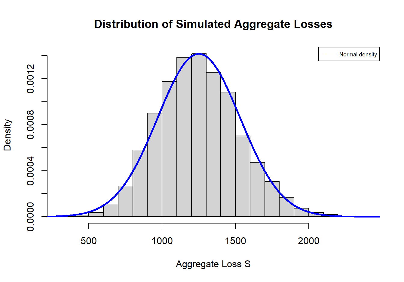
Example 5.4.2. Recall Example 5.3.5 with an individual’s claim frequency \(N\) has a Poisson distribution with mean \(\lambda=25\) and claim severity \(X\) is uniformly distributed on the interval \((5,95)\). Using a simulated sample of 10,000 observations, estimate the mean and variance of the aggregate loss \(S_N\). In addition, use the simulated sample to estimate the probability that aggregate claims for this individual will exceed 2,000 and compare with the normal approximation estimates from Example 5.3.5.

Show Example Solution

Solution. We follow the algorithm for the collective risk model, where we first simulate frequencies \(n_1,\ldots,n_{10000}\), and conditional on \(n_j,~j=1,\ldots,10000\), simulate each individual loss \(x_{ij},~i=1,\ldots n_j\).

set.seed(4321)  # For reproducibility of results
m <- 10000      # Number of observations to simulate
lambda <- 25    # Parameter for frequency distribution N
a <- 5; b <- 95 # Parameters for severity distribution X
S <- rep(NA, m) # Initialize an empty vector to store S observations

n <- rpois(m, lambda) # Generate m=10000 observations of N from Poisson
for(j in 1:m){ 
  n_j <- n[j] # Given each n_j (j=1,...,m), generate n_j observations of X from uniform
  x_j <- runif(n_j, min=a, max=b)
  s_j <- sum(x_j) # Calculate the aggregate loss s_j
  S[j] <- s_j # Store s_j in the vector of observations
}
mean(S) # Compare to theoretical value of 1,250

[1] 1248.09

var(S)  # Compare to theoretical value of 79,375

[1] 77441.22

mean(S>2000) # Proportion of simulated observations s_j that are > 2000

[1] 0.0062

# Compare to normal approximation method of 0.003884

Using simulation, we estimate the mean and variance of the aggregate claims to be approximately 1248 and 77441 respectively, compared to the theoretical values of 1,250 and 79,375. In addition, we estimate the probability that aggregate losses exceed 2000 to be 0.0062, compared to the normal approximation estimate of 0.003884.

We can assess the appropriateness of the normal approximation by comparing the empirical distribution of the simulated aggregate losses to the density of the normal distribution used for the normal approximation, \(N(\mu=1,250~, ~\sigma^2=79,375)\):

The simulated losses are slightly more right-skewed than the normal distribution, with a longer right tail. This explains why the normal approximation estimate of \(\Pr(S_N > 2000)\) is lower than the simulated estimate.

---

Show Quiz Solution

---

5.5 Effects of Coverage Modifications

5.5.1 Impact of Exposure on Frequency

This section focuses on an individual risk model for claim counts. Recall the individual risk model involves a fixed \(n\) number of contracts and independent loss random variables \(X_i\). Consider the number of claims from a group of \(n\) policies: \[S=X_1+\cdots+X_n ,\] where we assume \(X_i\) are iid representing the number of claims from policy \(i\). In this case, the exposure for the portfolio is \(n\), using policy as exposure base. In Section 7.4.1 we will introduce other exposure bases. The pgf of \(S\) is

\[ \begin{aligned} P_{S}(z)&={\rm E}(z^S)={\rm E}\left(z^{\sum_{i=1}^nX_i}\right)\\ &=\prod_{i=1}^n{\rm E}(z^{X_i})=[P_X(z)]^n . \end{aligned} \]

Special Case: Poisson. If \(X_i\sim Poi(\lambda)\), its pgf is \(P_X(z)=e^{\lambda(z-1)}\). Then the pgf of \(S\) is \[P_{S}(z)=[e^{\lambda(z-1)}]^n=e^{n\lambda(z-1)}.\] So \(S\sim Poi(n\lambda)\). That is, the sum of \(n\) independent Poisson random variables each with mean \(\lambda\) has a Poisson distribution with mean \(n\lambda\).

---

Special Case: Negative Binomial. If \(X_i\sim NB(\beta,r)\), its pgf is \(P_X(z)=[1-\beta(z-1)]^{-r}\). Then the pgf of \(S\) is \[P_{S}(z)=[[1-\beta(z-1)]^{-r}]^n=[1-\beta(z-1)]^{-nr}.\] So \(S\sim NB(\beta,nr)\).

---

Example 5.5.1. Assume that the number of claims for each vehicle is Poisson with mean \(\lambda\). Given the following data on the observed number of claims for each household, calculate the MLEMaximum likelihood estimate of \(\lambda\).

\[ {\small \begin{matrix} \begin{array}{c|c|c} \hline \text{Household ID} & \text{Number of vehicles} & \text{Number of claims} \\ \hline 1 & 2 & 0 \\ 2 & 1 & 2 \\ 3 & 3 & 2 \\ 4 & 1 & 0 \\ 5 & 1 & 1 \\ \hline \end{array} \end{matrix} } \]

Show Example Solution

Solution. Each of the 5 households has number of exposures \(n_j\) (number of vehicles) and number of claims \(S_j\), \(j=1,...,5\). Note for each household, the number of claims \(S_j \sim Poi (n_j \lambda)\). The likelihood function is
\[\begin{aligned} L(\lambda) &= \prod_{j=1}^5 \Pr(S_j=s_j) = \prod_{j=1}^5 \frac{e^{-n_j\lambda} (n_j \lambda)^{s_j}}{s_j!} \\ &= \left(\frac{e^{-2\lambda} (2 \lambda)^{0}}{0!} \right) \left(\frac{e^{-1\lambda} (1 \lambda)^{2}}{2!} \right) \left(\frac{e^{-3\lambda} (3 \lambda)^{2}}{2!} \right) \left(\frac{e^{-1\lambda} (1 \lambda)^{0}}{0!} \right) \left(\frac{e^{-1\lambda} (1 \lambda)^{1}}{1!} \right) \\ &\propto e^{-8\lambda} \lambda^5 \end{aligned}\] Taking the logarithm, we have \[\begin{aligned} l(\lambda) = \log L(\lambda) = -8\lambda + 5\log(\lambda) . \end{aligned}\] Setting the first derivative of the log-likelihood to 0, we get \(\hat{\lambda} = \frac{5}{8}\)

---

If the exposure of the portfolio changes from \(n_1\) to \(n_2\), we can establish the following relation between the aggregate claim counts: \[P_{S_{n_2}}(z)=[P_X(z)]^{n_2}=[P_X(z)^{n_1}]^{n_2/n_1}=P_{S_{n_1}}(z)^{n_2/n_1}.\]

5.5.2 Impact of Deductibles on Claim Frequency

This section examines the effect of deductibles on claim frequency. Intuitively, there will be fewer claims filed when a policy deductible is imposed because a loss below the deductible level may not result in a claim. Even if an insured does file a claim, this may not result in a payment by the policy, since the claim may be denied or the loss amount may ultimately be determined to be below deductible. Let \(N^L\) denote the number of losses (i.e. the number of claims with no deductible), and \(N^P\) denote the number of payments when a deductible \(d\) is imposed. Our goal is to identify the distribution of \(N^P\) given the distribution of \(N^L\). We show below that the relationship between \(N^L\) and \(N^P\) can be established within an aggregate risk model framework.

Note that sometimes changes in deductibles will affect policyholder claim behavior. We assume that this is not the case, i.e. the underlying distributions of losses for both frequency and severity remain unchanged when the deductible changes.

Given there are \(N^L\) losses, let \(X_1,X_2\ldots,X_{N^L}\) be the associated amount of losses. For \(j=1,\ldots,N^L\), define \[\begin{eqnarray*} I_j&=& \left \{ \begin{array}{cc} 1 & \text{if} ~X_j>d\\ 0 & \text{otherwise}\\ \end{array} \right.. \end{eqnarray*}\]

Then we establish \[N^P=I_1+I_2+\cdots+I_{N^L},\]

that is, the total number of payments is equal to the number of losses above the deductible level. Given that \(I_j\)’s are independent Bernoulli random variables with probability of success \(v=\Pr(X>d)\), the sum of a fixed number of such variables is then a binomial random variable. Thus, conditioning on \(N^L\), \(N^P\) has a binomial distribution, i.e. \(N^P | N^L \sim Bin(N^L, v)\), where \(v=\Pr(X>d)\). This implies that \[\begin{aligned} \mathrm{E}\left(z^{N^P}|N^L\right)&= \left[ 1+v(z-1)\right]^{N^L} \end{aligned}\]

So the pgf of \(N^P\) is \[\begin{aligned} P_{N^P}(z)&= \mathrm{E}_{N^P}\left(z^{N^P}\right)=\mathrm{E}_{N^L}\left[\mathrm{E}_{N^P}\left(z^{N^P}|N^L\right)\right]\\ &= \mathrm{E}_{N^L}\left[(1+v(z-1))^{N^L}\right]\\ &= P_{N^L}\left(1+v(z-1)\right) . \end{aligned}\]

Thus, we can write the pgf of \(N^P\) as the pgf of \(N^L\), evaluated at a new argument \(z^* = 1+v(z-1)\). That is, \(P_{N^P}(z)=P_{N^L}(z^*)\).

Special Cases:

• \(N^L\sim Poi (\lambda)\). The pgf of \(N^L\) is \(P_{N^L}=e^{\lambda(z-1)}\). Thus the pgf of \(N^P\) is \[\begin{aligned} P_{N^P}(z) &= e^{ \lambda(1+v(z-1)-1)} \\ &= e^{\lambda v(z-1)} , \end{aligned}\]
  So \(N^P \sim Poi(\lambda v)\). This means the number of payments has the same distribution as the number of losses, but with the expected number of payments equal to \(\lambda v = \lambda \Pr(X>d)\).

• \(N^L \sim NB(\beta, r)\). The pgf of \(N^L\) is \(P_{N^{L}}\left( z\right) =\left[ 1-\beta \left( z-1\right)\right]^{-r}\). Thus the pgf of \(N^P\) is \[\begin{aligned} P_{N^P}(z)&= \left( 1-\beta (1+v(z-1)-1)\right)^{-r}\\ &= \left( 1-\beta v(z-1)\right)^{-r}, \end{aligned}\] So \(N^P \sim NB(\beta v, r)\). This means the number of payments has the same distribution as the number of losses, but with parameters \(\beta v\) and \(r\).

---

Example 5.5.2. Suppose that loss amounts \(X_i\sim Pareto(\alpha=4,\ \theta=150)\). You are given that the loss frequency is \(N^L\sim Poi(\lambda)\) and the payment frequency distribution is \(N^{P}_1\sim Poi(0.4)\) at deductible level \(d_1=30\). Find the distribution of the payment frequency \(N^{P}_2\) when the deductible level is \(d_2=100\).

Show Example Solution

Solution. Because the loss frequency \(N^L\) is Poisson, we can relate the means of the loss distribution \(N^L\) and the first payment distribution \(N^{P}_1\) (under deductible \(d_1=30\)) through \(0.4 = \lambda v_1\), where \[\begin{aligned} &v_1 = \Pr(X > 30) = \left( \frac{150}{30+150}\right)^4=\left( \frac{5}{6}\right)^4 \\ \Rightarrow \ & \lambda = 0.4 \left( \frac{6}{5} \right)^4 . \end{aligned}\] With this, we can assess the second payment distribution \(N^{P}_2\) (under deductible \(d_2=100\)) as being Poisson with mean \(\lambda_2 = \lambda v_2\), where \[\begin{aligned} & v_2 = \Pr(X>100)=\left( \frac{150}{100+150}\right)^4=\left( \frac{3}{5}\right)^4 \\ \Rightarrow \ & \lambda_2 = \lambda v_2 = 0.4\left( \frac{6}{5} \right)^4 \left( \frac{3}{5} \right)^4 = 0.1075 . \end{aligned}\]

---

Example 5.5.3. Follow-Up. Now suppose instead that the loss frequency is \(N^L \sim NB(\beta,\ r)\) and for deductible \(d_1=30\), the payment frequency \(N^{P}_1\) is negative binomial with mean \(0.4\). Find the mean of the payment frequency \(N^{P}_2\) for deductible \(d_2=100\).

Show Example Solution

Solution. Because the loss frequency \(N^L\) is negative binomial, we can relate the parameter \(\beta\) of the \(N^L\) distribution and the parameter \(\beta_1\) of the first payment distribution \(N^{P}_1\) using \(\beta_1 = \beta v_1\), where \[v_1 = \Pr(X > 30) = \left( \frac{5}{6} \right)^4\] Thus, the mean of \(N^{P}_1\) and the mean of \(N^L\) are related via \[\begin{aligned} &0.4 = r \beta_1 = r \left(\beta v_1\right) \\ \Rightarrow \ & r\beta = \frac{0.4}{v_1} = 0.4 \left(\frac{6}{5} \right)^4 . \end{aligned}\] Note that \(v_2 = \Pr(X > 100) = \left( \frac{3}{5}\right)^4\) as in the original example. Then the second payment frequency distribution under deductible \(d_2=100\) is \(N^{P}_2 \sim NB(\beta v_2, \ r)\) with mean \[\begin{aligned} r (\beta v_2) = (r \beta) v_2 = 0.4 \left( \frac{6}{5}\right)^4 \left( \frac{3}{5} \right)^4 = 0.1075 . \end{aligned}\]

---

Next, we examine the more general case where \(N^L\) is a zero-modified distribution. Recall that a zero-modified distribution can be defined in terms of an unmodified one (as was shown in Section 2.5.1). That is, \[\begin{aligned} p_k^M = c~p_k^0, {~\rm for~} k=1,2,3,\ldots, {~\rm with~}c = \frac{1-p_0^M}{1-p_0^0}, \end{aligned}\] where \(p^0_k\) is the pmf of the unmodified distribution. In the case that \(p_0^M=0\), we call this a zero-truncated distribution, or \(ZT\). For other arbitrary values of \(p_0^M\), this is a zero-modified, or \(ZM\), distribution. The pgf for the modified distribution is shown as \[\begin{aligned} P^M(z) &= 1-c+c~P^0(z), \end{aligned}\] expressed in terms of the pgf of the unmodified distribution, \(P^0(z)\). When \(N^L\) follows a zero-modified distribution, the distribution of \(N^P\) is established using the same relation from earlier, \(P_{N^P}(z)=P_{N^L}\left(1+v(z-1)\right)\).

Special Cases:

• \(N^{L}\) is a ZM-Poisson random variable with parameters \(\lambda\) and \(p_0^{M}\). The pgf of \(N^L\) is \[P_{N^{L}}(z)=1-\cfrac{1-p_0^{M}}{1-e^{-\lambda}}+\cfrac{1-p_0^{M}}{1-e^{-\lambda}}\left( e^{\lambda(z-1)} \right).\] Thus the pgf of \(N^P\) is \[P_{N^{P}}(z)=1-\cfrac{1-p_0^{M}}{1-e^{-\lambda}}+\cfrac{1-p_0^{M}}{1-e^{-\lambda}}\left( e^{\lambda v(z-1)} \right).\] So the number of payments is also a ZM-Poisson distribution with parameters \(\lambda v\) and \(p_0^{M}\). The probability at zero can be evaluated using \({\rm Pr}(N^P=0) = P_{N^P}(0)\).

• \(N^{L}\) is a ZM-negative binomial random variable with parameters \(\beta\), \(r\), and \(p_0^{M}\). The pgf of \(N^L\) is \[P_{N^{L}}(z)=1-\cfrac{1-p_0^{M}}{1-(1+\beta)^{-r}}+\cfrac{1-p_0^{M}}{1-(1+\beta)^{-r}}\left[ 1-\beta \left( z-1\right)\right]^{-r}.\] Thus the pgf of \(N^P\) is \[P_{N^{P}}(z)=1-\cfrac{1-p_0^{M}}{1-(1+\beta)^{-r}}+\cfrac{1-p_0^{M}}{1-(1+\beta)^{-r}}\left[ 1-\beta v\left( z-1\right)\right]^{-r}.\] So the number of payments is also a ZM-negative binomial distribution with parameters \(\beta v\), \(r\), and \(p_0^{M}\). Similarly, the probability at zero can be evaluated using \({\rm Pr}(N^P=0) = P_{N^P}(0)\).

---

Example 5.5.4. Aggregate losses are modeled as follows:
(i) The number of losses follows a zero-modified Poisson distribution with \(\lambda=3\) and \(p_0^M = 0.5\).
(ii) The amount of each loss has a Burr distribution with \(\alpha=3, \theta=50, \gamma=1\).
(iii) There is a deductible of \(d=30\) on each loss.
(iv) The number of losses and the amounts of the losses are mutually independent.

Calculate \(\mathrm{E}(N^P)\) and \(\mathrm{Var}(N^P)\).

Show Example Solution

Solution. Since \(N^L\) follows a ZM-Poisson distribution with parameters \(\lambda\) and \(p_0^M\), we know that \(N^P\) also follows a ZM-Poisson distribution, but with parameters \(\lambda v\) and \(p_0^M\), where

\[v = \Pr(X>30) = \left( \frac{1}{1+(30/50)} \right)^3 = 0.2441 .\]

Thus, \(N^P\) follows a ZM-Poisson distribution with parameters \(\lambda^\ast = \lambda v= 0.7324\) and \(p_0^M = 0.5\). Finally, \[\begin{aligned} \mathrm{E} (N^P) &= (1-p_0^M) \frac{\lambda^\ast}{1-e^{-\lambda^\ast}} = 0.5 \left( \frac{0.7324}{1-e^{-0.7324}} \right) \\ &= 0.7053 \\ \mathrm{Var} (N^P) &= (1-p_0^M) \left( \frac{\lambda^\ast[1-(\lambda^\ast + 1) e^{-\lambda^\ast}]}{(1-e^{-\lambda^\ast})^2} \right) + p_0^M(1-p_0^M) \left(\frac{\lambda^\ast}{1-e^{-\lambda^\ast}} \right)^2 \\ &= 0.5 \left( \frac{0.7324(1-1.7324 e^{-0.7324})}{(1-e^{-0.7324})^2} \right) + 0.5^2 \left( \frac{0.7324}{1-e^{-0.7324}} \right)^2 \\ &= 0.7244 . \end{aligned}\]

---

5.5.3 Impact of Policy Modifications on Aggregate Claims

In this section, we examine how a change in the deductible affects the aggregate payments from an insurance portfolio. We assume that the presence of policy limitsA policy limit is the maximum value covered by a policy. (\(u\)), coinsuranceCoinsurance is an arrangement whereby the insured and insurer share the covered losses. typically, a coinsurance parameter specified means that both parties receive a proportional share, e.g., 50%, of the loss. (\(\alpha\)), and inflation (\(r\)) have no effect on the underlying distribution of frequency of payments made by an insurer. As in the previous section, we further assume that deductible changes do not impact the underlying distributions of losses for both frequency and severity.

Recall the notation \(N^L\) for the number of losses. With ground-up lossThe total amount of loss sustained before policy adjustments are made (i.e. before deductions are applied for coinsurance, deductibles, and/or policy limits.) amount \(X\) and policy deductible \(d\), we use \(N^P\) for the number of payments (as defined in the previous section 5.5.2). Also, define the amount of payment on a per-loss basisDue to policy modifications (e.g. deductibles), not all losses that occur result in payment. the per-loss basis considers every loss that occurs. as \[\begin{eqnarray*} X^{L}&=\left\{ \begin{array}{ll} 0 ~, & \text{if } ~X<\cfrac{d}{1+r} \\ \alpha[(1+r)X-d]~, & \text{if } ~\cfrac{d}{1+r}\leq X<\cfrac{u}{1+r} \\ \alpha(u-d)~, & \text{if } ~X \ge \cfrac{u}{1+r}\\ \end{array} \right., \end{eqnarray*}\] and the amount of payment on a per-payment basisDue to policy modifications (e.g. deductibles), not all losses that occur result in payment. the per-payment basis which considers only the losses that result in some payment to the insured. as \[\begin{eqnarray*} X^{P}&=\left\{ \begin{array}{ll} {\rm undefined} ~, & \text{if }~ X<\cfrac{d}{1+r} \\ \alpha[(1+r)X-d]~, & \text{if }~ \cfrac{d}{1+r}\leq X<\cfrac{u}{1+r} \\ \alpha(u-d)~, & \text{if } ~ X \ge \cfrac{u}{1+r} .\\ \end{array} \right.. \end{eqnarray*}\] In the above, \(r\), \(u\), and \(\alpha\) represent the inflation rate, policy limit, and coinsurance, respectively. Hence, aggregate costs (payment amounts) can be expressed either on a per loss or per payment basis:

\[ \begin{aligned} S &= X^L_1 + \cdots + X^L_{N^L} \\ &=X^P_1 + \cdots + X^P_{N^P} ~. \end{aligned} \]

(Recall that when we introduced the per-loss and per-payment bases in Section 3.4, we used another letter \(Y\) to distinguish losses from insurance payments, or claims. At this point in our development, we use the letter \(X\) to reduce notation complexity.)

The fundamentals regarding collective risk models are ready to apply. For instance, we have: \[\begin{aligned} {\rm E}(S) &= {\rm E}\left(N^L\right) {\rm E}\left(X^L\right) = {\rm E}\left(N^P\right) {\rm E}\left(X^P\right)\\ {\rm Var}(S) &= {\rm E}\left(N^L\right) {\rm Var}\left(X^L\right) + \left[{\rm E}\left(X^L\right)\right]^2 {\rm Var}(N^L) \\ &= {\rm E}\left(N^P\right) {\rm Var}\left(X^P\right) + \left[{\rm E}\left(X^P\right)\right]^2 {\rm Var}(N^P)\\ M_S(z)&=P_{N^L}\left[M_{X^L}(z)\right]=P_{N^P}\left[M_{X^P}(z)\right] . \end{aligned}\]

---

Example 5.5.5. Actuarial Exam Question. A group dental policy has a negative binomial claim count distribution with mean 300 and variance 800. Ground-up severity is given by the following table:

\[ {\small \begin{matrix} \begin{array}{ c | c } \hline \text{Severity} & \text{Probability}\\ \hline 40 & 0.25\\ 80 & 0.25\\ 120 & 0.25\\ 200 & 0.25\\ \hline \end{array} \end{matrix} } \]

You expect severity to increase 50% with no change in frequency. You decide to impose a per claim deductible of 100. Calculate the expected total claim payment \(S\) after these changes.

Show Example Solution

Solution. The cost per loss with a 50% increase in severity and a 100 deductible per claim is \[\begin{eqnarray*} X^L &=& \left\{ \begin{array}{cc} 0 & 1.5x<100 \\ 1.5x-100 & 1.5x\ge 100\\ \end{array} \right. \end{eqnarray*}\] This has expectation \[\begin{aligned} \mathrm{E}(X^L) &= \frac{1}{4} \left[ \left(1.5(40)-100\right)_+ + \left(1.5(80)-100\right)_+ + \left(1.5(120)-100\right)_+ + \left(1.5(200)-100\right)_+ \right] \\ &= \frac{1}{4}\left[ (60-100)_+ + (120-100)_+ + (180-100)_+ + (300-100)_+\right] \\ &= \frac{1}{4}\left[ 0 + 20 + 80 + 200 \right] = 75 . \end{aligned}\] Thus, the expected aggregate loss is \[\mathrm{E}(S)=\mathrm{E}(N) ~ \mathrm{E} \left(X^L \right)= 300 (75) = 22,500 . .\]

---

Example 5.5.6. Follow-Up. What is the variance of the total claim payment, \(\mathrm{Var~}(S)\)?

Show Example Solution

Solution. On a per loss basis, we have \[\begin{aligned} \mathrm{Var}(S) &= \mathrm{E}(N) ~ \mathrm{Var}\left( X^L \right) + \left[ \mathrm{E} \left(X^L\right) \right]^2 ~ \mathrm{Var} (N) \end{aligned}\] where \(\mathrm{E}(N) = 300\) and \(\mathrm{Var}(N) = 800\). We find \[\begin{aligned} &\mathrm{E} \left[ (X^L)^2 \right] = \frac{1}{4} \left[ 0^2 + 20^2 + 80^2 + 200^2 \right] = 11,700 \\ \Rightarrow \ & \mathrm{Var}(X^L) = \mathrm{E} \left[ (X^L)^2 \right] - \left[ \mathrm{E}(X^L) \right]^2 = 11,700 - 75^2 = 6,075 \end{aligned}\] Thus, the variance of the aggregate claim payment is \[\begin{aligned} \mathrm{Var}(S) &= 300(6,075) + 75^2 (800) = 6,322,500 . \end{aligned}\]

---

Alternative Method: Using the Per Payment Basis. Previously, we calculated the expected total claim payment by multiplying the expected number of losses by the expected payment per loss. Recall that we can also multiply the expected number of payments by the expected payment per payment. In this case, we have \[S=X_1^P + \cdots + X_{N_P}^P \] The probability of a payment is \[\Pr(1.5X \ge 100)=\Pr(X \ge 66.\bar{6})=\frac{3}{4} .\] Thus, the number of payments, \(N^P\) has a negative binomial distribution (see negative binomial special case in Section 5.5.2) with mean \[\mathrm{E}(N^P) = \mathrm{E}(N^L)~\Pr(1.5X \geq 100) = 300 \left(\frac{3}{4} \right)=225 .\] The cost per payment is \[\begin{eqnarray*} X^P &=& \left\{ \begin{array}{ll} \text{undefined}~, & \text{if }~ 1.5x<100 \\ 1.5x-100~, & \text{if } ~ 1.5x\ge 100\\ \end{array} \right. \end{eqnarray*}\] This has expectation \[\mathrm{E}(X^P)=\frac{\mathrm{E}(X^L)}{\Pr(1.5X > 100)}=\frac{75}{(3/4)}=100 .\] Thus, as before, the expected aggregate loss is \[\mathrm{E}(S)=\mathrm{E}(X^P) ~ \mathrm{E}(N^P) = 100(225)=22,500 .\]

---

Example 5.5.7. Actuarial Exam Question. A company insures a fleet of vehicles. Aggregate losses have a compound Poisson distribution. The expected number of losses is 20. Loss amounts, regardless of vehicle type, have exponential distribution with \(\theta=200\). To reduce the cost of the insurance, two modifications are to be made:
(i) A certain type of vehicle will not be insured. It is estimated that this will reduce loss frequency by 20\(\%\).
(ii) A deductible of 100 per loss will be imposed.

Calculate the expected aggregate amount paid by the insurer after the modifications.

Show Example Solution

Solution. On a per loss basis, we have a 100 deductible. Thus, the expectation per loss is \[\begin{aligned} \mathrm{E}( X^L) &= E[(X-100)_+] = E(X) - E(X\wedge 100) \\ &= 200 - 200(1-e^{-100/200}) = 121.31 . \end{aligned}\] Loss frequency has been reduced by 20\(\%\), resulting in an expected number of losses \[\mathrm{E}(N^L) = 0.8(20) = 16 .\] Thus, the expected aggregate amount paid after the modifications is \[\mathrm{E}(S) = \mathrm{E}(X^L)~ \mathrm{E} (N^L) = 121.31(16) = 1,941\]

---

Alternative Method: Using the Per Payment Basis. We can also use the per payment basis to find the expected aggregate amount paid after the modifications. With the deductible of 100, the probability that a payment occurs is \(\Pr(X > 100) = e^{-100/200}\). For the per payment severity, plugging in the expression for \(\mathrm{E}(X^L)\) from the original example, we have \[\begin{aligned} \mathrm{E} (X^P) = \frac{\mathrm{E} (X^L)}{\Pr(X > 100)} = \frac{200 - 200(1-e^{-100/200})}{e^{-100/200}} = 200 \end{aligned}\] This is not surprising – recall that the exponential distribution is memorylessThe memoryless property means that a given probability distribution is independent of its history and what has already elapsed. specifically, random variable x is memoryless if pr(x > s+t | x >= s) = pr(x > t). note that it does not mean x > s+t and x >= s are independent events., so the expected claim amount paid in excess of 100 is still exponential with mean 200.

Now we look at the payment frequency \[\mathrm{E} (N^P) = \mathrm{E}(N^L)~\Pr(X>100) = 16 ~e^{-100/200} = 9.7.\] Putting this together, we produce the same answer using the per payment basis as the per loss basis from earlier \[\mathrm{E}(S) = \mathrm{E} (X^P)~ \mathrm{E} (N^P)= 200(9.7) = 1,941.\]

---

Show Quiz Solution

---

5.6 Further Resources and Contributors

5.6.0.1 Exercises

Here are a set of exercises that guide the viewer through some of the theoretical foundations of Loss Data Analytics. Each tutorial is based on one or more questions from the professional actuarial examinations, typically the Society of Actuaries Exam C/STAM.

Aggregate Loss Guided Tutorials

Contributors

• Peng Shi and Lisa Gao, University of Wisconsin-Madison, are the principal authors of the initial version of this chapter. Email: pshi@bus.wisc.edu for chapter comments and suggested improvements.
• Chapter reviewers include: Vytaras Brazauskas, Mark Maxwell, Jiadong Ren, Sherly Paola Alfonso Sanchez, and Di (Cindy) Xu.

TS 5.A.1. Individual Risk Model Properties

For the expected value of the aggregate loss under the individual risk model,

\[\begin{aligned} \mathrm{E}(S_n) &=\sum_{i=1}^n ~ \mathrm{E}(X_i) = \sum_{i=1}^n ~ \mathrm{E}(I_i \times B_i) = \sum_{i=1}^n ~ \mathrm{E}(I_i) ~~ \mathrm{E}(B_i) ~~~~ \text{from the independence of } I_i \text{'s and } B_i \text{'s} \\ &= \sum_{i=1}^n \Pr(I_i=1) ~ \mu_i ~~~~ \text{since the expectation of an indicator variable is the probability it equals } 1 \\ &= \sum_{i=1}^n ~ q_i ~ \mu_i . \end{aligned}\]

For the variance of the aggregate loss under the individual risk model,

\[\begin{aligned} \mathrm{Var}(S_n) &= \sum_{i=1}^n \mathrm{Var}(X_i) ~~~~ \text{from the independence of } X_i \text{'s} \\ &= \sum_{i=1}^n ~ \left( ~ \mathrm{E}\left[ \mathrm{Var}(X_i | I_i) \right] + \mathrm{Var}\left[ \mathrm{E}(X_i|I_i) \right] ~ \right) ~~~~ \text{from the conditional variance formulas} \\ &= \sum_{i=1}^n \left( q_i ~ \sigma_i^2 ~ + ~ q_i ~ (1-q_i) ~ \mu_i^2 \right) . \end{aligned}\]

To see this, note that \[\begin{aligned} \mathrm{E}\left[ \mathrm{Var}(X_i | I_i) \right] &= \mathrm{Var}(X_i|I_i=0) ~ \Pr(I_i=0) + \mathrm{Var}(X_i|I_i=1) ~ \Pr(I_i=1) \\ &= q_i ~ \sigma_i^2 + (1-q_i) ~ (0) = q_i ~ \sigma_i^2, \end{aligned}\]

and \[\begin{aligned} \mathrm{Var}\left[ \mathrm{E}(X_i|I_i) \right] &= q_i ~ (1-q_i) ~ \mu_i^2~, \end{aligned}\]

using the Bernoulli variance shortcut since \(\mathrm{E}(X_i|I_i) = 0\) when \(I_i=0\) (probability \(\Pr(I_i=0) = 1-q_i\)) and \(\mathrm{E}(X_i|I_i) = \mu_i\) when \(I_i=1\) (probability \(\Pr(I_i=1)= q_i\)).

For the probability generating function of the aggregate loss under the individual risk model,

\[ \begin{aligned} P_{S_n}(z) &= \prod_{i=1}^n ~ P_{X_i}(z) ~~~~ \text{from the independence of } X_i \text{'s} \\ &= \prod_{i=1}^n ~ \mathrm{E}(z^{~X_i}) = \prod_{i=1}^n ~ \mathrm{E}(z^{~I_i \times B_i}) = \prod_{i=1}^n ~\mathrm{E} \left[ \mathrm{E}(z^{~I_i \times B_i} | I_i) \right] ~~~~ \text{from the law of iterated expectations} \\ &= \prod_{i=1}^n \left[ ~ E\left(z^{~I_i \times B_i} | I_i=0\right) ~ \Pr(I_i=0) + E\left(z^{~I_i \times B_i} | I_i=1\right) ~ \Pr(I_i=1) ~ \right] \\ &= \prod_{i=1}^n ~ \left[ ~ (1) ~ (1-q_i) + P_{B_i}(z) ~ q_i ~ \right] = \prod_{i=1}^n \left(~ 1-q_i + q_i ~ P_{B_i}(z) ~\right) \end{aligned} \]

Lastly, for the moment generating function of the aggregate loss under the individual risk model,

\[ \begin{aligned} M_{S_n}(t) &= \prod_{i=1}^n ~ M_{X_i}(t) ~~~~ \text{from the independence of } X_i \text{'s} \\ &= \prod_{i=1}^n ~ \mathrm{E}(e^{t~X_i}) = \prod_{i=1}^n ~ \mathrm{E}\left(e^{~t~(I_i \times B_i)} \right) \\ & = \prod_{i=1}^n ~ \mathrm{E} \left[ \mathrm{E} \left( e^{~t~(I_i \times B_i)} | I_i \right) \right] ~~~~ \text{from the law of iterated expectations} \\ &= \prod_{i=1}^n ~ \left[~ \mathrm{E}\left(e^{~t~(I_i \times B_i)} | I_i=0 \right) ~ \Pr(I_i=0) + \mathrm{E}\left( e^{~t~(I_i \times B_i)} | I_i=1 \right) ~ \Pr(I_i=1) ~\right] \\ &= \prod_{i=1}^n ~ \left[ ~ (1) ~ (1-q_i) + M_{B_i}(t) ~ q_i ~ \right] = \prod_{i=1}^n \left(~ 1-q_i + q_i ~ M_{B_i}(t) ~\right) . \end{aligned} \]

---

TS 5.A.2. Relationship Between Probability Generating Functions of \(X_i\) and \(X_i^T\)

Let \(X_i\) belong to the \((a,b,0)\) class with pmf \(p_{ik} = \Pr(X_i = k)\) for \(k=0,1,\ldots\) and \(X_i^T\) be the associated zero-truncated distribution in the \((a,b,1)\) class with pmf \(p_{ik}^T = p_{ik}/(1-p_{i0})\) for \(k=1,2,\ldots\). Then the relationship between the pgf of \(X_i\) and the pgf of \(X_i^T\) is shown by

\[\begin{aligned} P_{X_i}(z) &= \mathrm{E~}(z^{X_i}) = \mathrm{E}\left[ \mathrm{E}\left( z^{X_i} | X_i \right) \right] ~~~~ \text{from the law of iterated expectations} \\ &= \mathrm{E}\left( z^{X_i} | X_i=0 \right)~ \Pr(X_i=0) + \mathrm{E}\left( z^{X_i} | X_i>0 \right) ~ \Pr(X_i>0) \\ &= (1)~ p_{i0} + \mathrm{E}(z^{X_i^T}) ~ (1-p_{i0}) ~~~~ \text{since } (X_i | X_i>0) \text{ is the zero-truncated random variable } X_i^T \\ &= p_{i0} +(1-p_{i0}) P_{X_i^{T}}(z) . \end{aligned}\]

---

TS 5.A.3. Example 5.3.8 Moment Generating Function of Aggregate Loss \(S_N\)

For \(N\sim Geo(\beta)\) and \(X\sim Exp(\theta)\), we have

\[ \begin{aligned} P_N (z) &=\frac{1}{1- \beta (z-1)}\\ M_{X}(t) &=\frac{1}{1-\theta t} . \end{aligned} \]

Thus, the mgf of aggregate loss \(S_N\) is

\[ \begin{aligned} M_{S_N}(t) &= P_N [M_{X}(t)] = \frac{1}{1 - \beta \left( \frac{1}{1-\theta t} - 1\right)} \\ &= \frac{1}{1 - \beta \left( \frac{\theta t}{1-\theta t} \right)} + 1 - 1 = 1+ \frac{\beta \left( \frac{\theta t}{1-\theta t} \right)}{1 - \beta \left( \frac{\theta t}{1-\theta t} \right)} \\ &= 1 + \frac{\beta \theta t}{(1-\theta t) - \beta \theta t} = 1+ \frac{\beta \theta t}{1-\theta t (1+\beta)} \cdot \frac{1+\beta}{1+\beta} \\ &= 1 + \frac{\beta}{1+\beta} \left[ \frac{\theta (1+\beta) t}{1-\theta(1+\beta)t} \right] \\ &= 1 + \frac{\beta}{1+\beta} \left[ \frac{1}{1-\theta(1+\beta)t} - 1 \right], \\ \end{aligned} \]

which gives the expression (5.1). For the alternate expression of the mgf (5.2), we continue from where we just left off:

\[ \begin{aligned} M_{S_N}(t) &= 1 + \frac{\beta}{1+\beta} \left[ \frac{\theta (1+\beta) t}{1-\theta(1+\beta)t} \right] \\ &= \frac{1+\beta}{1+\beta} + \frac{\beta}{1+\beta} \left[ \frac{\theta (1+\beta) t}{1-\theta(1+\beta)t} \right] \\ &= \frac{1}{1+\beta} + \frac{\beta}{1+\beta} + \frac{\beta}{1+\beta} \left[ \frac{\theta (1+\beta) t}{1-\theta(1+\beta)t} \right] \\ &= \frac{1}{1+\beta} + \frac{\beta}{1+\beta}\left[1 + \frac{\theta (1+\beta) t}{1-\theta (1+\beta)t} \right] \\ &= \frac{1}{1+\beta} +\frac{\beta}{1+\beta} \left[ \frac{1}{1-\theta (1+\beta)t}\right] . \end{aligned} \]